![]()
![]()
![]()
![]()
![]()
![]()
![]()
![]()
visual transport modeller: mode choice model
![]()
Back to version 2 walkthroughs On to Distribution models Mode choice models model the travellers choice of which mode of transport to take e.g. car or any public transport. They take as input variables about each possible mode of transport that the traveller has available for the trip, and gives the proportion of travellers which would use each mode of transport. (e.g. 70% by car and 30% by public transport).
If a trip matrix were input into the mode choice model, it would split the matrix into separated matrices, one for each mode of transport. (For this reason it is sometimes called a mode split model.) These matrices can be assigned to the highway and public transport networks respectively to give flows on each section of highway or each public transport service.
If individual trips are input into the mode choice model (e.g. trips obtained from a household interview survey), then the mode choice model will provide the probability of this trip using each mode of transport. If the trip record has an expansion factor which represents the total number of people with this choice, then the mode choice model will apply the probability to the expansion factor to give the expanded number of people who chose each mode of transport.
Input Data
The modeller must decide which variables are relevant to the decision making process but the most common variables for urban and interurban travel are: in-vehicle time, walk time, wait time, cost and how many interchanges are involved. This data can be 'skimmed' from the highway and public transport networks for each origin-destination pair to form matrices, which are called skims because they are obtained by skimming along the paths accumulating the data.
The modeller must also determine which modes are available - or the choice set. This is sometimes not so easy but Visual-tm will provide this as a skim, which will be covered later.
Mode Choice Modelling using Visual-tm
In order to demonstrate matrix based mode choice modelling we will start by opening the Ashtest project. If you use the Dataviewer to investigate the network data files stored, you can see that there are 2 modes of transport loaded. These are road and rail, (ie. car and PT). Lets concentrate on the Car Available Work (CAW) market segment. The observed mode split, taken and expanded from market research is: -
Mode No of trips Mode share (%) Car 45499 99.00% Bus 459 1.00% Total 45958 100.00% The aim at this stage is to calibrate a model that predicts a mode split very similar to that shown above i.e. it accurately portrays the current situation.
When conducting a Modal Choice exercise there are three key elements. These are: -
Skims a skim is a matrix containing an attribute, one matrix for each attribute, for each mode i.e. 2 modes, 7 attributes = 14 skims.
Utility Function Coefficients these multiply the attribute to form the utility function.
Trip Matrix this holds the number of trips by all modes between each origin and destination. This matrix is to be split by the mode choice model into one matrix for each mode of transport using the utility functions and logit model described earlier. To do this it has to have the attribute for each mode for each attribute for each o-d pair (these are provided by the skims) and the utility function coefficients.
Each of these will now be discussed in turn.
Skimming
A skim is a matrix containing a variable value for each zone to zone movement in the study area. Visual-tm has 2 methods for producing skims. You can skim for individual attributes separately or we have pre-programmed a standard set of skims, however this is not as versatile as getting the skims individually. These are generated through the assignment procedure. In order to demonstrate this particular feature you will need to open the Ashtest data set. Click Models/Assignment to open the form below:
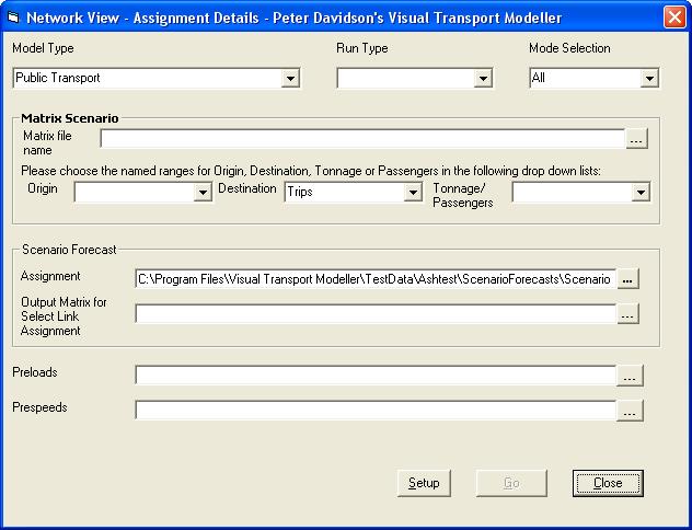
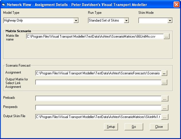
Select the Model Type i.e. Highway Only, Public Transport or Park and Ride, Public Transport and Highway. Then in Run Type select Standard Set of Skims and then and then select the mode that you wish to skim for. A text box labelled Output Skim File is now available at the bottom of the form. You can enter a name for the output skim file here. If no name is entered, the skim file will be called pbSkim.dat and will be in the projects \System\Working directory.
Select an input matrix. For skimming purposes if you need to generate skim values for all o-d pairs, you simply need to input an n x n unit matrix (pre-filled with 1) where n is the number of zones. The unit matrix must be in Binary Erica Trips or Comma Separated Variable Format. If it is in Binary Erica Trips format, select the Market segment number that includes the data, and Trips from the drop down menu.
Now click Setup, which will open the form below:
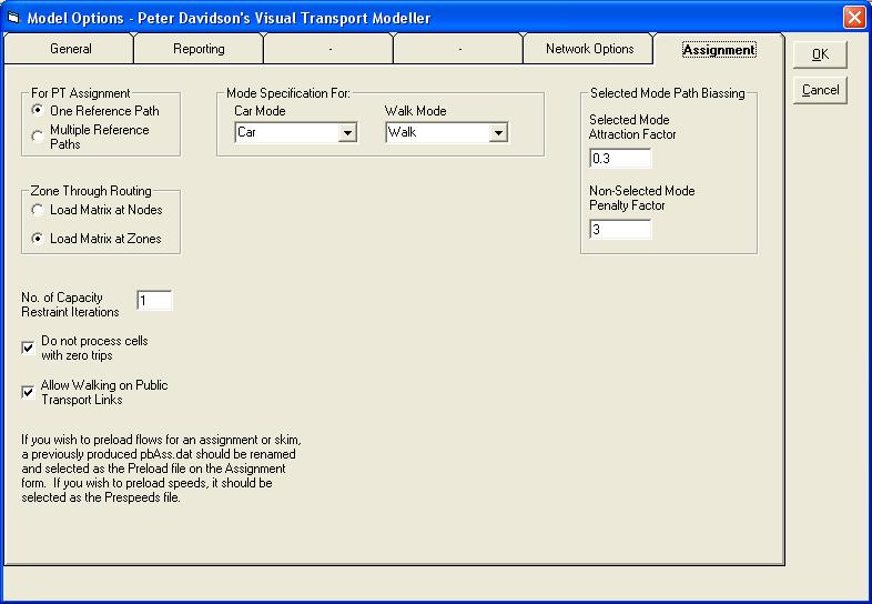
Firstly on this form you need to select the car mode and walk modes from the drop down lists. If the project has modes called Car and Walk, these will be put in automatically. The final option is to set the total number of zones and the number of internal zones on the General tab. In the Ashford project this is 66 and 37 respectively.
If you wish to preload flows for an assignment or skim, a previously produced pbAss.dat should be selected in the Preloads text box. If you wish to preload speeds, it should be entered as the Prespeeds File. For this example, we are not using preloads.
Click OK to confirm the settings, which will return you to the Assignment run form. Click Go to run the skimming process.
This facility has been pre-programmed to provide a full set of skims in the following format for each mode. Unless a file name has been specified as explained above, this file will be called pbskim.dat and will be output to the system/working directory of your active project.
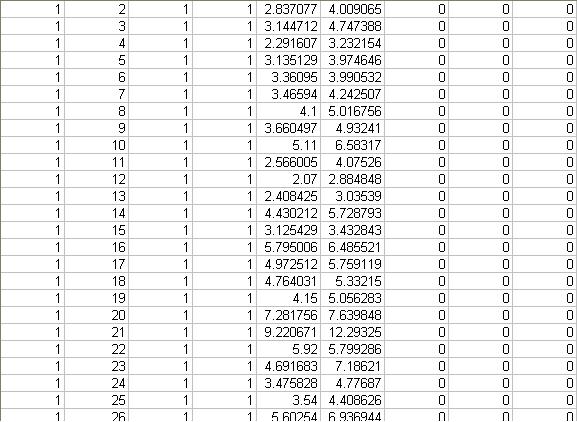
The columns in the file shown above are Origin Zone, Destination Zone, Mode Available, Mode Constant, Cost, In Vehicle Time, Wait time, Walk time, no of Interchanges.
Coeffiecients
In laymans terms, coefficients are weighting factors that tell the mode choice system how much emphasis to place on each associated cost. They can differ greatly from region to region. For example in a very affluent area it is likely that the most important factor when making a mode choice decision is the length of time taken to make the journey whereas in a much poorer area, cost may be the most important factor.
The coefficient files themselves are stored in a text format with a file extension of .pdo. They can be viewed and edited using a text-editing package such as Brief, WordPad or Notepad.
Lets have a look at one of the coefficient files. The base coefficients for the CAW market segment are called CoeffMchoiCAW.pdo and are stored in Skims/Calibration/CAW. Open the file using your text-editing package.
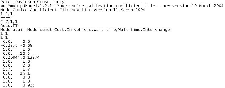
In this section of the Walkthrough we will explain the structure of these files, however, the coefficient values themselves will not be discussed. Coefficient values can be derived with Stated Preference Market Research. PDC has a wealth of experience in this field and currently holds an extensive library of coefficients that have been obtained through stated preference market research.
The first four lines are headers and version information that give the purpose of the file and the coefficient file version and the fifth line separates this information from the start of the actual data.
The sixth line gives 4 numbers 2,7,1,1 (x,y,a,b) Where: - x = No of modes y = No of market segments in the skim file. a = No of times the full set of coefficients is repeated in the file b = No of calibration areas (always set to 1)
The seventh line gives the two modes in order. This order is important and should be remembered for when attempting the mode choice model run.
The eighth line gives the attribute titles, which should be the same for all modes. Again the order is important.
The ninth and tenth lines contain information for nested logit models. Currently both of these need to have a 1 for each mode of transport.
The eleventh and twelfth rows are scaling factors to scale the relative coefficients to match the observed mode shares. The twelfth row is the In Vehicle Time Coefficient.
On the thirteenth line the coefficients start. The structure of the coefficients is shown below: -
Attribute 1 Mode 1 Attribute 1 Mode 2 Attribute 2 Mode 1 Attribute 2 Mode 2 Attribute 3 Mode 1 Attribute 3 Mode 2 Attribute 4 Mode 1 Attribute 4 Mode 2 Attribute 5 Mode 1 Attribute 5 Mode 2 Attribute 6 Mode 1 Attribute 6 Mode 2 Attribute 7 Mode 1 Attribute 7 Mode 2 Commas are used to separate the values.
The row following the coefficients should always have as many zeroes on it as there are modes.
The final two rows are Calibration factors. These are output from mode choice calibration and the user should set these to unity to start with.
Running the Mode Split
In Visual Transport Modeller there are a number of options/methods of running a mode split. These depend upon the format of your input matrix and what outputs are required from the model run. The method we will discuss here is where the user has a simple trip matrix stored in Comma Separated Variable format and the objective is to split this trip matrix into one matrix for each mode.
On the main Visual-tm form Click Models/Mode Choice and then choose the Matrix option. This opens the Mode Choice Run Control Form shown below.
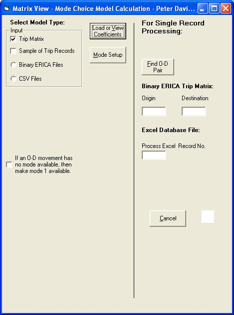
Click the Load or View Coefficients button to open the form below.
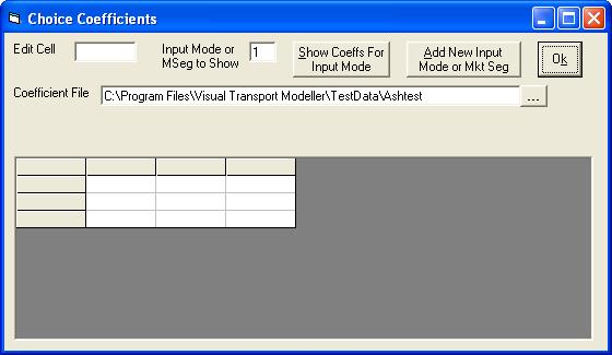
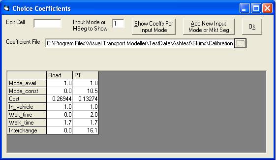
Browse to the CoeffMchoiCAW.pdo file stored in Skims/Calibration/CAW. Select and Click Open. This will redisplay the Mode Choice Run Control Form (click OK to close it):
For this type of mode choice run, the Model Type is a trip matrix in CSV format. Make sure that this box and option button (and only these) are selected. There are two modes in the Ashtest project, so enter 2 into the No. of Modes text box.
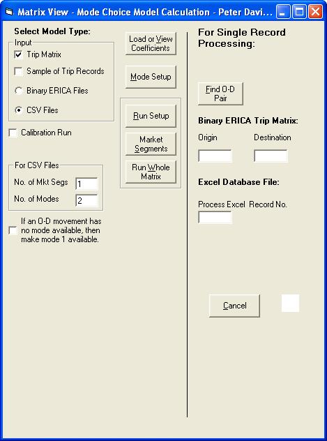
If the Mode Available attribute is set to No for all the modes for a given O-D pair, the trips will not be allocated to any of the output matrices. This may be prevented, if desired, by clicking the check box labelled If an O-D movement has no mode available, then make mode 1 available. This will assign all the trips for the O-D pair to the first mode. There are no such O-D pairs in this test data set but this can be an issue when for example running a mode choice model on a non car available market segment, depending upon how you have configured your network. Best practice is to code your network so that there is at least one mode available for each o-d movement.
Click Run Setup and the form below will open.
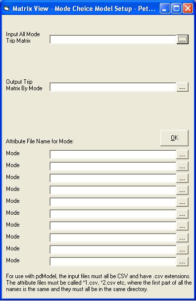
This is the main form where you set the parameters for your model run.
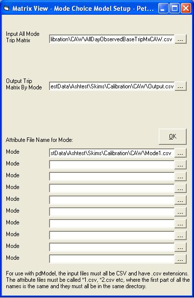
Because we are calculating base mode split we will use the base input trip matrix. This file is called AllDayObservedBaseTripMxCAW.csv and is stored under in the same folder as the coefficient file.
We have provided an Output matrix trip file. It is called Output.csv and is saved in the same location.
We now need to allocate the skim files for each mode we have created. It is essential that the skim files are input in the same order as the modes were set up in the coefficients file i.e. Car; PT.
The skims must all be in the same directory and have names of the form *1.csv, *2.csv etc. These must also be in the correct order and the *1.csv file should be entered in the first skim file text box. The rest do not need to be entered as the program derives their names.
Click the button to browse and select the first skim file. You can either use the ones you have created during previous sessions of this Walkthrough or alternatively we have stored complete skim files called Mode1.csv and Mode2.csv.
For a simple trip matrix mode split this form is now completed and should look like this.
Click OK to close the form and save.
We are now ready to perform the mode split. To do this click Run Whole Matrix.
Once finished, the total numbers of trips allocated to each mode are given on the form.
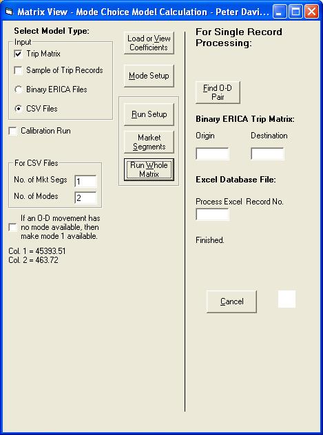
Lets now compare these figures with the observed mode split we mentioned earlier.
Observed Forecast No of Trips Mode Share No of Trips Mode Share Mode Car 45499 99.00% 45394 98.99% PT 459 1.00% 464 1.01% Total 45958 100.00% 45858 100.00% As you can see the model predicts a mode split that accurately portrays the observed situation. Therefore our first objective has been met.
Back to version 2 walkthroughs On to Distribution models