![]()
![]()
![]()
![]()
![]()
![]()
![]()
![]()
visual transport modeller: networks
![]()
Back to version 2 walkthroughs On to Public transport On to Checking paths All the data needed to build a network is contained in a spreadsheet. In the Astest test data project the file for the base network is ScenarioNetworks\Base\Road.xls. Every network is made up of nodes and links. The nodes usually represent junctions and stations and the links represent highway or rail. The network is plotted by the software as shown.
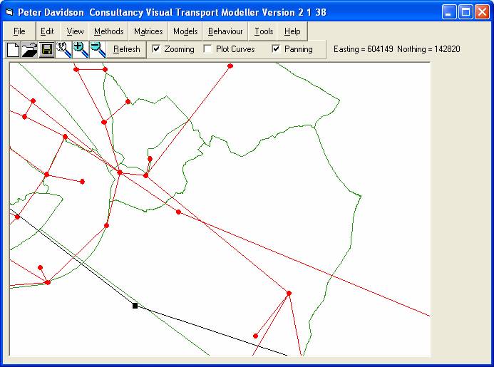
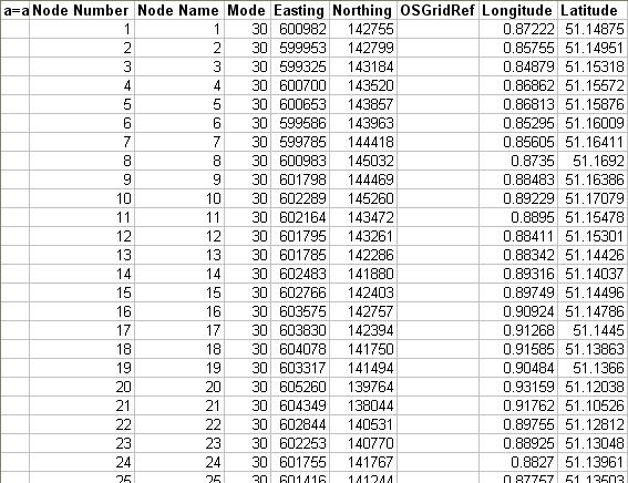
Nodes
The nodes are given a name, a number and a mode. The mode depends on whether it is a highway node, rail node or zone centroid, for example. Their grid reference can be obtained by plotting the nodes on the map (Select 'Map' from the 'View' menu).
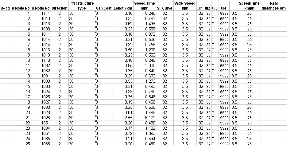
Links
Links connect the nodes together. Highway links obviously connect highway nodes, rail links connect rail nodes and zone connectors connect any type of node to the zone centroids. The length of each link can be found using the route planner command on the map. The speed flow curve of the link also needs to be specified.
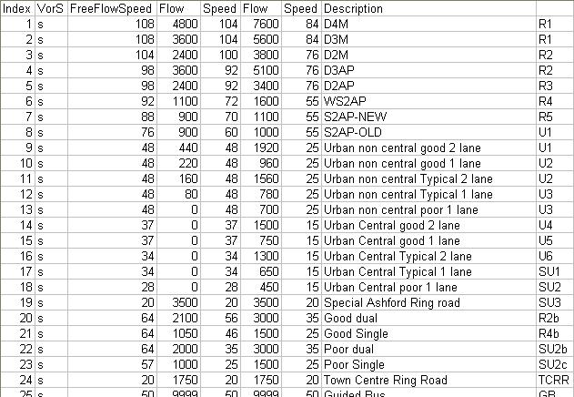
Speed Flow Curves
All the necessary speed flow curves are entered into the functions sheet of the Road.xls workbook. Each curve needs an index number, its free flow speed, its flow at free flow speed, the lowest speed at which it can maintain that flow, the capacity of the link and the speed at capacity.
In order to check that the speed flow curves of the network are accurate you must first of all assign a matrix with the values of all of the traffic movements and only assign a single iteration to this Assignment. You will be given an Assignment.xls file with the flows and the speeds and this needs to be copied and saved in a separate folder to be referred to for future reference. You then need to reassign this data but add an extra iteration and the data will change so that the flows and speeds compensate for the differences to the predicted speed flow curve i.e. if the flow was large after the second iteration the flow will decrease and the speed will increase. You then need to save the new Assignment.xls and keep reassigning the matrix with an extra iteration each time until the flows and speeds seem to be reaching a constant value.
In Road.xls you can then make your own calibration speed flow curve from the data held in the functions section and the SF number given in the Links section. To do this you match the SF number given for the route between the two links to the set of speeds and flows in the Links section and make a graph of these two sets of numbers (speed vs. flow). After the line finishes the curve goes into an asymptote downwards from the edge of the curve. The formula for this Asymptote is as follows:
Where V is the speed at the demand flow that you want the software to calculate. Vc is the speed at the maximum flow (the last speed in the SF data). L is the link length. e is the flow of the traffic that is in Assignment.xls divided by the flow at capacity, given in the data about the SF curve.

On this graph you can then plot where the speed and the flow of a particular link is and if this plot is not at its maximum speed for this flow then this means that the speed can increase and this can be plotted on the graph. The speed in Assignment.xls should be equal to the speed predicted by the curve at the flow that the Assignment has given. If the flow is above the capacity flow then it should match the speed predicted by the formula given above. However once the speed has increased then the link will become more attractive to use and so become more congested and will get a larger flow in the next iteration. This will result in the speed on the graph decreasing to the level shown on the SF Curve. This in turn will result in a decrease in the speed so an increase in the flow on the next iteration and so on. This will then lead to a spiral in the graph that will eventually settle at the speed and flow that the link should be at with all the movements from the matrix.

In order to check that the software is making any changes in the speeds and flows if the flows are large enough, you can look in 'Pd-ModelLogfile.dat' where you can view the number of links that have changed by a certain speed.

To check that the software is functioning correctly you can run a different number of iterations of the data when assigning your matrix to get the varying flows and speeds of the traffic. To do this you just run the Assignment as before in the path building and where it asks for the number of capacity restraint iterations you enter 2 or more in this box. The eventual speed and flow of the graph should be the same as that predicted by the software.
When these iterations are entered, the flows and speeds between these links will be different than the previous iteration as it will have reassigned to eventually, after enough iterations, make the speed and flow equal to the final value obtained on the SF Curve. To view the individual changes in the flow and speed of the two links you can look in Assignment.xls under the headings 'totals' and 'speed' and view them along with the general cost between the two links. The flows can also be viewed in 'PbAss.dat' where the flows are given in the fourth column of numbers. You can run the assignment iteration as many times as is necessary to get a suitable result for the SF Curve. However usually it is not necessary to check after the second iteration of the flow and speed as the problems will normally show up by the first and second iterations.
In the file Road.xls you can see the free flow speed, the time it takes to go between links and the distance between them. You can also view the changes in the flows of certain links by going to 'pd-ModelLogfile.dat' and viewing the figures highlighted below which show the speed changes and the amount of links which have changed by this amount.
Back to version 2 walkthroughs On to Public transport On to Checking paths