Mode Choice Modelling Using Visual-TM

Matrix based mode choice

If we have a trip matrix then we can split it into trip matrices for each mode of transport by considering each movement (or matrix cell) from one origin to one destination in turn. The calculation is the same as above: calculate the utility, exponentiate it, sum over all modes and calculate the proportion by each mode, apply these proportions to the trip matrix to give the number of trips for each mode and write these out to the matrix for each mode. This calculation is then repeated for each origin to destination zone pair in the trip matrix to give the trip matrix for each mode.

In order to demonstrate matrix based mode choice modelling we will use the Performance Test Data.

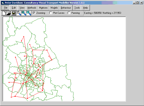
Open the Performance Data project (below)

If you use the Dataviewer to investigate the network data files stored, you can see that there are 5 modes of transport loaded.  These are: -

Road                                                                                                                                                                                          Bus                                                                                                                                                                                  Cycle                                                                                                                                                                           Quality Bus                                                                                                                                                                      Walk

Although the Quality Bus network is occasionally currently in operation, we will use the normal bus network for our calibration exercise.

The observed mode split, taken and expanded from market research is: -

The aim at this stage is to calibrate a model that predicts a mode split very similar to that shown above i.e. it accurately portrays the current situation.

We have also pre-loaded 3 additional scenario options for your use.  These are: -

1. A Trend forecast for 2010.  

Congestion levels have increased along with the number of trips.  Nothing else has altered.  This will answer the question “What will the mode share be like in 2010 if we do nothing?”

2. A Local Transport Plan forecast for 2010

Congestion levels have increased along with the number of trips.  However to combat this we have fully introduced the Quality bus scheme by buying new buses and implementing bus and cycle priority ways in some areas of the town.

3. An Additional Measures Forecast for 2010.

On top of the LTP measures we have also doubled the bus frequency and implemented even more cycle ways enabling a 10% increase in cycle speed.

Preparation

When conducting a Modal Choice exercise there are three key elements.  These are: -

Each of these will now be discussed in turn.

 Skimming

A skim is a matrix containing a variable value for each zone to zone movement in the study area.  We have different associated variables for each mode of transport.

Visual TM has 2 methods for producing skims.  You can skim for individual attributes separately or we have pre-programmed a standard set of skims.  

Lets initially look at the variables we have attributed to the modes of transport.  They are shown in the table below.

In this example, skim files are Binary Erica – Trip matrices and each file can hold several matrices where there is an attribute in each matrix.

As you can see Market Segments 1 and 2 are for Mode Available and Mode Constant respectively.  In this example they are both pre-filled with a value of one: -

So for example the car mode skim file is to be structured like this: -

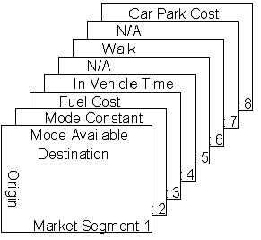
When a cost for a specific mode is Not Applicable (N/A) instead of a skim file you simply need to enter a n x n unit matrix (pre-filled with 1’s) where n = No. of Zones.

One way to create this file is to create a single attribute matrix file for each cost for each mode and then interleave the matrices using the Matrix Manipulation functionality of pd-Edit.

An easier (although less versatile way) is to skim a standard set of skims from the network, one set for each mode – this is discussed later. Some skims however, are generated through external sources.  For example Bus Fare charge is a charge that is not easily allocated to links.  These cost matrices should be obtained through local means and saved or converted into a n x n Binary Erica – Trip matrix using pd-Edit where n = No. of Zones.  In the test data these skim files have been provided.

Skims that are derived through the network (in the Performance Test Data example are shown in the table below.

Next we will look at how the network skim files are calculated.  What basically happens here is that the system will calculate the shortest path between all zones in the network then add all the associated costs together to generate a skim value for each o-d pair.

i.e.  Zone 1 to 2 Road fuel cost skim.

In order to run the skimming process it is generally best to create the files that are needed prior to the run.  These have been created for you.  Lets concentrate on the Car skims file.

To conduct the skimming process it is essential that the correct network scenario be built.  Use the Dataviewer to build the base car network.

Once the base car network is built Click Models/Attribute Skims and the form below appears

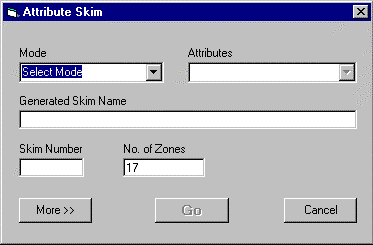
In the Select Mode drop down list, select road.

In the Select Attribute drop down list, select price.

The generated Skim Name field is automatically filled in.

Because we are building single market segment matrices, the skim number is 1.

There are 12 zones in the Performance test data so enter 12 in the No. of Zones field.

Click More >> and the form expands as shown below

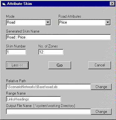
The Relative Path and Range Name field are automatically entered.

You need to select an output file.  These files have been created in the directory Skims Folder Manual/Completed/Carskims.  Click Change and browse to this directory.  Select the CarPrice.bmt file and select Open.

The controls are now set.  Click Go to run the skim.

When it has finished, the form displays the Skim Complete message.

Now do the Car IVT skim.

There is no need to close the form. In the Road Attributes drop down list, select IVT.

The Output file needs to be changed.  Click change and browse to the same directory select the CarIVT.bmt file

Click Go to run the skim.

This procedure should now be followed for all the network skim files for each mode but you must: -

Remember to build the correct mode network before running the skim

Remember to put the number of zones at 12

Remember to change the output file

Remember to set the Skim Number at 1

Once you have created these individual skim files (you should have 8 for each mode) it is now time to manipulate them together.  This is done using the interleaving functions of pd-Edit.

On the Matrix menu click Matrix Calculations and then Interleave to display the form below.

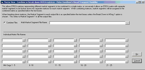
This form is pretty self-explanatory.  Let’s merge the car skims.  The Multi-Market Segment file has been provided and is called CarSkims.bmt.  It is stored in the same location as the individual car skim matrices.

Click   and browse to this file.  Select and Click Open.

At the bottom of the screen the individual matrices now need to be entered.  

Click   and browse to the files.  Select and Click Open.  

It is essential that the order of the skim files is the same as that shown earlier (and below).  When a cost is N/A simply select a UnitMX file as the individual matrix file.  These UnitMX files are simple 12 x 12 matrices pre-filled with the value of 1.

When completed the car skims interleave form should look like this.

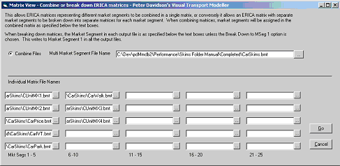
Click Go to interleave the matrices.

Now repeat this process for the other 3 modes.

For the base scenario, the skimming process is now completed.  Skimming will need to be repeated to generate skim files for each of the scenarios.  Simply follow the guidelines above, remembering to have the correct network built when running a network skim.  For example when calculating the bus skims for the LTP and Additional Measures scenario, make sure that you build the Quality Bus Network rather than the normal bus.

Alternatively, if you feel confident that you understand the principle of skimming, you can use the skim files that have been created and provided with the test data.  A complete set of skim files for each scenario is stored under Skims Folder Manual/Mode Choice 2000.

Entering data in network files for skimming is discussed under Network Data/Links in Section 5.4.2.

Before we move to the next section and discuss coefficients we can work out a short cut way of getting a standard set of skims, however this is not as versatile as getting the skims individually:

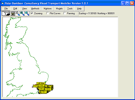
Visual TM has been pre-programmed to produce a standard set of skims.  These are generated through the assignment procedure.  In order to demonstrate this particular feature you will need to open the Ashford test data set shown below

Click Models/Assignment to open the form below

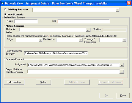
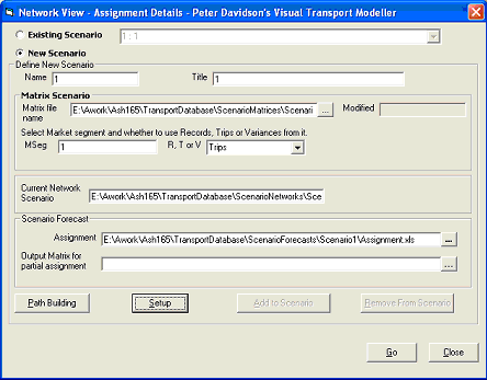
Define a new Scenario Name and title and select an input matrix.  For skimming purposes if you need to generate skim values for all o-d pairs, you simply need to input an n x n unit matrix (pre-filled with 1) where n is the number of zones in Binary Erica Trips Format.  Now select the Market segment number that includes the data, in this case 1 and Trips from the drop down menu.  Now click Setup, which will open the form below:

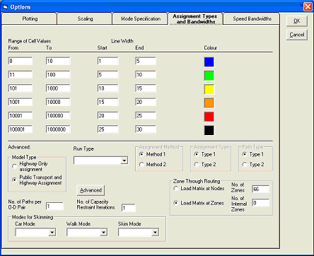
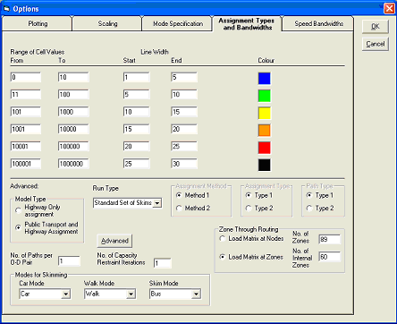
Firstly on this form select the Model Type i.e. Highway or Public Transport.  Then in Run Type select Standard Set of Skims.  If you are skimming the highway network you only need to select the car mode and walk modes from the drop down lists.  If you are skimming PT you also need to select which PT mode you want to skim for.  I.e. Bus.  The final option is to set the total number of zones and the number of internal zones.  In the Ashford project this is 66 and 37 respectively.  The completed form for a bus PT skim should look like this

Click OK to confirm the settings, which will return you to the Assignment run form.  This form should now look like this:

Click Go to run the skimming process.  

This facility has been pre-programmed to provide a full set of skims in the following format for each mode.  This file will be output in .csv format, called pbskim.dat and will be output to the system/working directory of your active project.  It can be converted into Binary Erica format using pd-Edit.

We have covered the 2 different methods of skimming included in Visual TM.  We can now move on to investigate the next key element of mode choice modelling, Mode Choice Coefficients.