![]()
![]()
![]()
![]()
![]()
![]()
![]()
![]()
Visual-tm: The Transport Database
![]()
Back to tutorials On to networks Covered in this section:
- Project data structure
- The system files
- Navigating the databases
- Adding, deleting and modifying data
- Data manipulation tools
Project data structure
Data is stored in Visual-tm in a simple hierarchical way. There are up to ten levels of databases, each level may have a number of databases contained within. In this documentation it is assumed that the databases are stored as MS Excel spreadsheet files; however it is also possible to store data in MS Access or CSV form.
Network data will be used as an example to fully explain the hierarchical structure. Data will be stored as follows. Navigation around the databases is facilitated by defining relevant pathnames to the next level of database. The coming example will therefore only mention the database name and relevant pathname field. Other information such as installation date and language are contained within the database file, but are not of concern here.
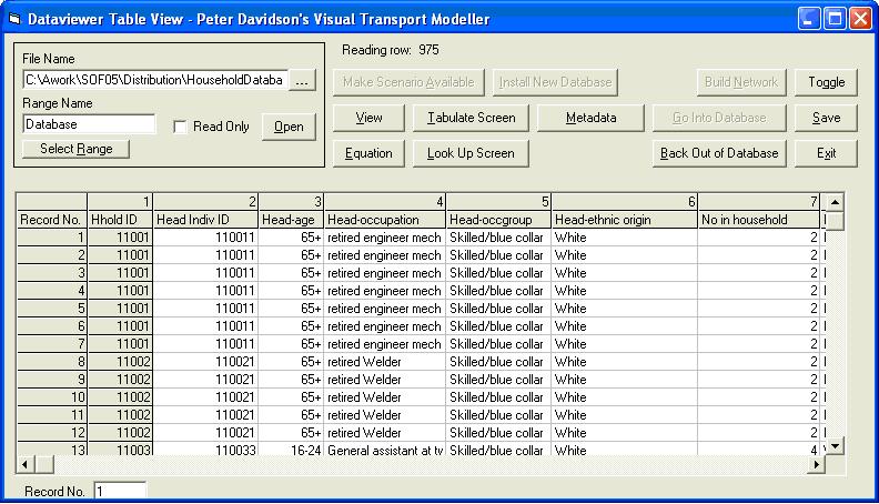
It may assist you to browse through the relevant files in the test data. Using the Dataviewer you can navigate through the databases by clicking on the relevant pathname field for your desired database followed by clicking on the Go Into Database button. Similarly, to return click the Back Out of Database button. To open the Dataviewer select Database from the View menu:
It is also worth mentioning at this stage that you will not see the full pathname to the particular file. What you actually see is the path from the project folder directory, i.e. the system assumes the files are stored within your project folder.
For example, the NetworkList.xls file, which is included with the test data, is actually stored:
C:\Program Files\Peter Davidson Consultancy\Visual-tm\TestData\Ashtest\ScenarioNetworks\NetworkList.xls
Whereas the system only shows:
\ScenarioNetworks\NetworkList.xls
Database files also contain range names, which enable the system to read specific information from each spreadsheet. A further description of range names is given in chapter 8.
The following descriptions are of files in the Ashtest project. Use the Dataviewer to follow this sequence.
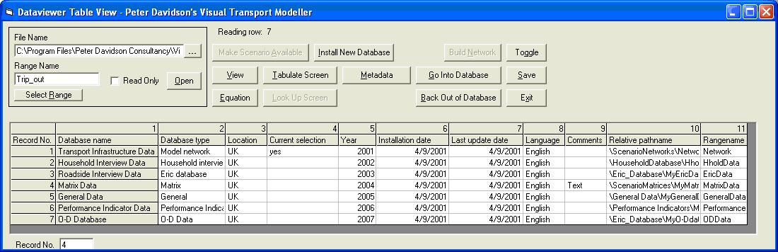
Databases_loaded.xls
This file is the top-level database and contains links to all other areas for storing data. It is structured as below:
Database name Relative pathname Range name Transport Infrastructure Data \ScenarioNetworks\NetworkList.xls Network Household Interview Data \Household Database\HholdProj.xls HholdData Roadside Interview Data \Eric_Database\MyEricDatabase.xls EricData Matrix Data \ScenarioMatrices\MyMatrixDatabase.xls MatrixData General Data \General Data\MyGeneralData.xls GeneralData Performance Indicator Data \Performance Indicators\MyPerformanceIndicators.xls Performance O-D Database \Eric_Database\MyO-Ddata.xls ODData Select the Transport Infrastructure Data Relative Pathname field and click Go Into Database. This now opens NetworkList.xls.
NetworkList.xls
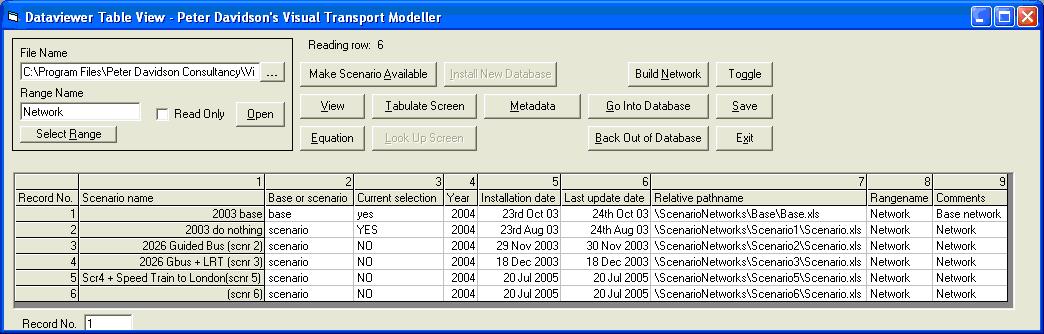
This is a second level database and contains information relating to the network infrastructure. It shows links to the base network files (the top line) followed by links to your scenario networks. Visual-tm requires that you have a do nothing scenario, which is usually given as Scenario 1. You can have as many other scenarios as required (Ashtest has a further five scenarios). The file is structured as below:
Scenario name Relative pathname Range name 2003 base \ScenarioNetworks\Base\Base.xls Network 2003 do nothing \ScenarioNetworks\Scenario1\Scenario.xls Network 2026 Guided bus (scnr 2) \ScenarioNetworks\Scenario2\Scenario.xls Network 2026 Gbus + LRT (scnr 3) \ScenarioNetworks\Scenario3\Scenario.xls Network Scr4 + Speed Train to London (scnr 5) \ScenarioNetworks\Scenario5\Scenario.xls Network (scnr 6) \ScenarioNetworks\Scenario6\Scenario.xls Network Select the base network relative pathname field and click Go Into Database. This now opens the base.xls file.
Base.xls/Scenario.xls
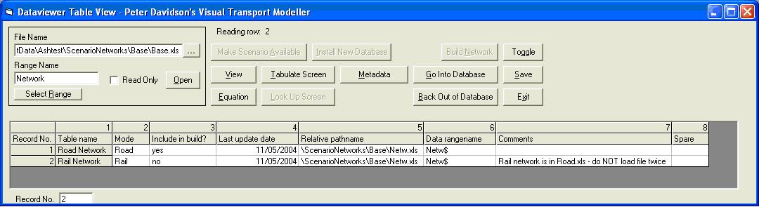
These files are the third level of database and contain the links to the Netw.xls files that point to the data. There may be a different Netw.xls file for each mode, but it is acceptable to have the data for all modes in the same spreadsheet in which case one Netw.xls file is sufficient. These files are structured as below:
Table name Relative pathname Range name Road network \ScenarioNetworks\Base\Netw.xls Netw Rail network \ScenarioNetworks\Base\Netw.xls Netw Select the road network relative pathname and click Go Into Database. This will now open the Netw.xls file.
Netw.xls
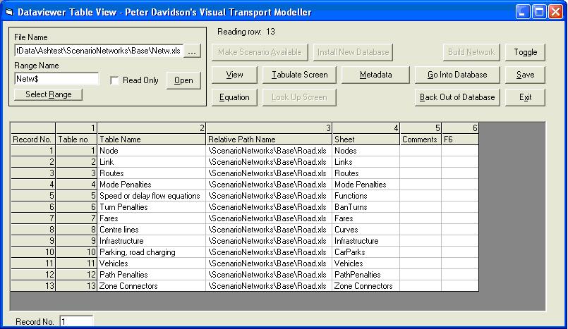
The Netw.xls files allow the different data types to be stored in separate files for the same mode, which is required for Comma Separated Variable network data. For network data in Excel files, it makes more sense to have all the data for a mode in one file as the ScenarioComponent.xls file in the Templates directory from which the mode network spreadsheets are derived is designed for this.
These files are the fourth level of database and contain the links to your actual mode network files. Each mode needs to have a file or files containing Node, Zone and Link information. There may also be optional extra data such as banned turns and public transport routes and fares. The data is always held on a sheet called Netw and these files are structured as below:
etc.
Table name Relative pathname Sheet Node \ScenarioNetworks\Base\Road.xls Nodes Link \ScenarioNetworks\Base\Road.xls Links Routes \ScenarioNetworks\Base\Road.xls Routes Thirteen different data types are specified in the file, of which the first three are shown above. The Table names must always be exactly as specified in the file as the software looks for these names in the file when loading the network. The Nodes and Links data are in ranges with the names as specified and the rest of the data types are on sheets with the names as specified. If any of the data is in comma separated variable files, there is no need to enter anything in the Sheet column beside its name.
Selecting any of the tables and clicking Go into Database will display the selected table.
The Road.xls file is the lowest level of database contained within the network data. It contains all the information relevant to building your base mode network. When viewing the file through the Dataviewer, the area of the spreadsheet which is actually shown is governed by range names or will be the part of the named sheet that has had data entered on it.
The system files
Every Visual-tm project contains a directory called System\Working. This directory contains system files. None of the files in this folder should be edited unless specifically stated.
Databases_loaded.xls
This file shows the relative pathnames to the files shown at the top level of the Dataviewer.World.mif
This is a MapInfo Interchange Format file. It is used to plot the background zone system in the Network display. It can be viewed and edited using a text-editing package such as Brief or WordPad. Please see the screenshot below.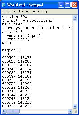
The .mif file basically contains some initial drawing instructions at the very top, which can be copied for any other project.
It then contains the polygon information. As you can see above, the first polygon is called Region 1 and has 207 points. These points are then listed below as OSGR Easting and Northing co-ordinates.
The drawing of the map is very straightforward. Firstly a line is drawn between the first and second set of co-ordinates. The end point of this line is then connected to the third co-ordinate; the end of this line is then connected to the fourth co-ordinate and so on. The key point to remember is that the first co-ordinate and the last co-ordinate in the list must be identical so that the polygon is a complete shape.
Each polygon is then listed in turn with the co-ordinates of its points. The polygons should fit together with no overlaps or gaps to cover the entire geographical area of study.
Navigating the databases
To open the Dataviewer simply click View/Database on the main Visual-tm form.
The Dataviewer operates within Visual-tm where it holds the actual data as a consistent set of databases. It provides tools for viewing, editing, adding additional fields, tabulating and outputting data.
The databases comprise data tables in a hierarchical data structure with up to ten levels of data table, each level nested within the next level in the hierarchy. The nesting is also branched to other tables so that a table at one level can point to many tables at the next level down. Each record in the table can have a field containing a path and filename of the data table at the next level down that the user can go into.
To navigate through the data tables simply click on any cell in the row with the database that you wish to view, then click Go Into Database. Click Back Out of Database to reverse.
The project tree
The quickest and easiest way to view the complete data structure within a project is to use the project data structure form. Choose Project Tree from the View menu to open it.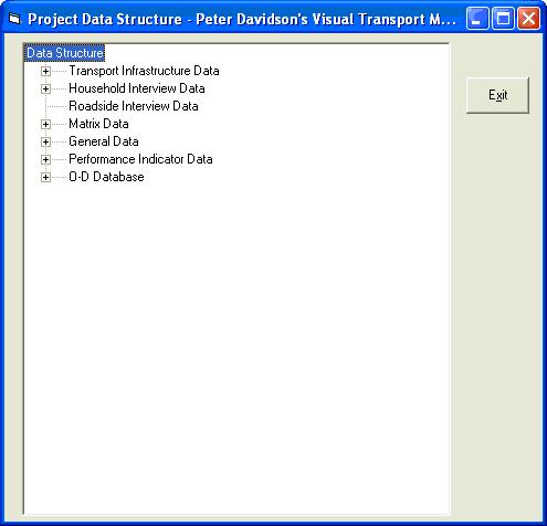
In this form you can currently see the databases loaded into this project. Simply click on the
signs to expand further.
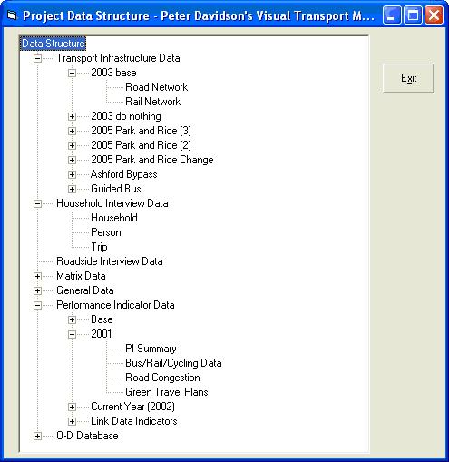
You can double click on a specific data item to open the Dataviewer and display the data that was selected.
Adding, deleting and modifying data
Editing data through the Dataviewer is achieved by clicking the View Button. This opens the View form (below). Here you can simply edit data stored in any of the records by typing the required changes into the fields. Use the Record Navigator section at the bottom right to choose which record and which field you wish to edit.
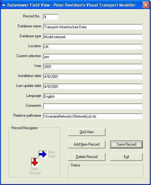
You can also Add New Records or Delete Existing Records by clicking on the appropriate button on the View form. Remember to click Save Record to save any changes made when exiting. You must also click Save on the Dataviewer form to save the changes to the file. Click Exit to return to the Dataviewer without saving changes.
Using the Dataviewer it is possible to open many types of file, even if they are not included in your nested hierarchy structure. At the top left corner of the Dataviewer you can click on the
button to browse to your required file. Select the appropriate range name and click open. This file can then be edited and viewed in the way described above.
Data manipulation tools
Lookup
The Dataviewer provides the facilities for manipulating variables through set parameters. This is achieved by applying named ranges to a chosen set of variables and storing them in your HHI data table.Lets investigate the HHI test data. Open the Ashtest test data set and use the Dataviewer to open the trips level data table of the household interview data (below)
If we look at the main mode of trip and main mode number columns there were 12 options for the interviewee. These and their relative codes are shown below:
1 = Car
2 = Car Passenger
3 = Car Share
4 = Work Bus
5 = Public Bus
6 = Bicycle
7 = Walk
8 = Underground
9 = Train
10 = Taxi
11 = Motorbike
12 = OtherIt is very unlikely that all 12 of these modes would be of interest in a multi-modal modelling project. These modes can actually be squeezed down to just 5 modes, for example:
1 = Car
2 = Walk
3 = Cycle
4 = Bus
5 = TrainThe squeeze pattern for these codes would be:
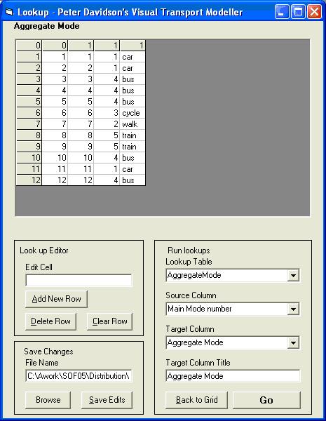
Original Code Aggregate Code Aggregate Mode 1 1 Car 2 1 Car 3 4 Bus 4 4 Bus 5 4 Bus 6 3 Cycle 7 2 Walk 8 5 Train 9 5 Train 10 4 Bus 11 1 Car 12 1 Bus This squeeze pattern has been saved to the HHI datatable and called AggregateMode.
Once the trips level data has loaded click the Look Up Screen button. The form below appears.
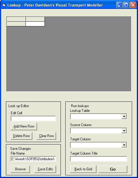
In the Run Lookups section of the screen select the Lookup Table to use as Aggregate Mode. At the top of the screen you can now see the squeeze pattern just mentioned.
The Source Column should be the un-squeezed mode column in the trips data table. This is Main Mode number.
The Target Column should be the destination you wish the Aggregate Mode code to be output to. An Aggregate Mode column has been added to the trips data table for this purpose. The completed form should look like this:
Now click Go to run the Lookup. When completed a message saying Aggregation Complete is displayed. Click Back to Grid to view the trips data table with the new entries in the Aggregate Mode column (below)
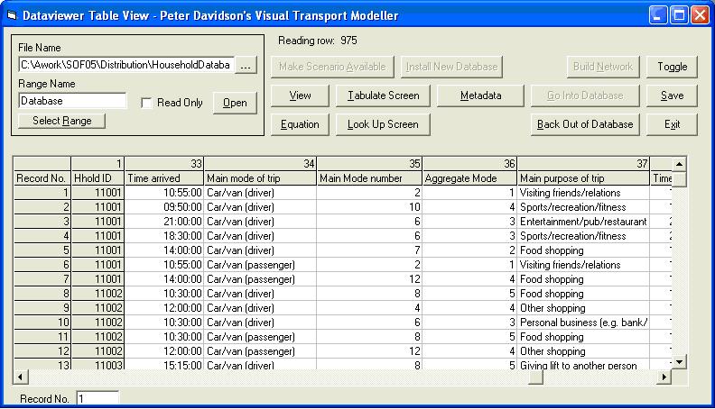
Click Save in the Dataviewer to save the changes back to the spreadsheet for additional editing or analysis.
As you can imagine, Lookup can be quite a complex tool to set up but the functionality it provides can be invaluable to the transport planner.
Tabulation
The Dataviewer provides the functionality required to tabulate some of your transportation data. This is an important tool and can be very useful, particularly when attempting to analyse large data files with possibly several thousands of records. The Dataviewer also provides the capability to export and save your tabulated data to an MS Excel spreadsheet, which can then be used in external applications.In order to demonstrate this, lets have a look at the household interview person level data. Open the Dataviewer and navigate so this data table is open (below).
There are 132 records in this file. Say for instance you want to generate a profile of the ages of people who were interviewed in each ward. Manually this would be a painstaking process. The tabulate facility makes it quick and easy. Click Tabulate Screen and the form below opens.

At the top left of this new screen you are asked to select which variables you wish to tabulate. The options to choose from are taken directly from the headings of the data table you wish to tabulate. In this example select the Person range from the drop down menu under the file name. Choose Household District as the Vertical axis and Age as the horizontal axis. The Dataviewer also enables the user to apply weighting and expansion factors to the tabulated data. These are optional and are not required for this example (they are described later in this section). Now click Tabulate.
The system now initialises the tabulation process. This can take a few minutes depending upon the processing power of your CPU and the complexity of your data table. Once completed the tabulated database appears (below).

Click Show values to display the age groups and Ward names as shown below.

Saving your tabulation is a simple process. At the top right of the Tabulation form click to display the Open File dialogue box. Either enter a new filename or browse to your required Excel spreadsheet file (in which case you should also select a sheet name from the drop down menu) and click Save to Excel. The table is then saved below any previous tabulation outputs that have been saved to that file.
Weighting and expansion factors
If your data contains columns with weighting factors or expansion factors which correspond to the columns you select in the Vertical axis or Horizontal axis box, then these can be selected from the relevant drop down menu. The records will be multiplied by these values before they are displayed in the table.Simple tabulation of whole range into Excel file
The tick box Simple Tabulation of whole range into Excel file will output a simple count of the entries in every column of your data to the Excel file you select in the top right of the form. It is not necessary to fill in the Horizontal and Vertical axes boxes, simply choose the you want tabulated from the box under the filename, enter the name of your Excel file, tick the box and click the Tabulate button.
Back to tutorials On to networks