![]()
![]()
![]()
![]()
![]()
![]()
![]()
![]()
Back to tutorials On to assignment models Covered in this section:
- Address Matching
- Zone Coding
- Rezoning RSI data
- Reversing RSI data
- RSI Expansion
- Market segmentation in your Excel data
- The parameter files
- RSI Matrix building
- RSI Matrix outputs
- Other data matrix building
- Overall build specification
Address Matching
Trips in Visual Transport Modeller are defined as an origin destination pair, where origin is the originating zone of the trip and destination is the destination zone of the trip. We discussed zone systems earlier in the Data section of this manual.
Our task here is to allocate zone numbers to the trips we have collected in our market research. The first stage of this process is address matching.
As you can imagine, when trip information is gathered it is most likely that actual addresses or postcodes will be collected. We need to convert these postcodes into Ordnance Survey Grid References (OSGRs). This is done using Visual-tms Address Matcher along with the Royal Mail Postal Address Finder Database (in the UK). The Address Matcher enables the user to quickly allocate OSGRs to postcodes or addresses. This can be done one address at a time or a batch file can be used.
This element of the software is not part of the standard installation of Visual-tm, plus there are licence requirements linked to the Postal Address Finder Database. Therefore this aspect will not be covered further in this tutorial. Please contact PDC for any further information.
Zone coding
Having allocated OSGR co-ordinates to the trips recorded in our market research, the next stage is to calculate the zones these co-ordinates fall into. This is achieved using the Address Zone Coder. In order to undertake this task you need a digitised zonal system in .mif format, an MS Excel file with Zone Names, an MS Excel file with your trip data provided as OSGR coordinates. Examples of these files are included in the Ashtest test data set.
Open the test data and click Methods/Address Zone Coding. The form below appears.
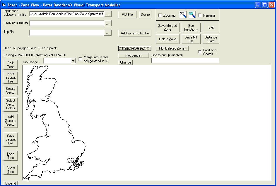
The Input zone polygons file is called The Final Zone System.mif and is stored in the Admin Boundaries directory.
Click
and browse to the file, select and click Open. Now click Plot File followed by Remove Deletions. The zone system is drawn at the bottom of the screen:
The Input Zone Names file is called Zonenames.xls stored in the same location. Click
The Trip file is called Trips.xls stored in the same location. I would suggest viewing this file prior to running the Address Zone Coder so you can identify outputs from the software. Notice that currently the columns Origin_Zone and Destination_Zone are empty. Remember to close the file once viewed. On the Address Zone Coder form click
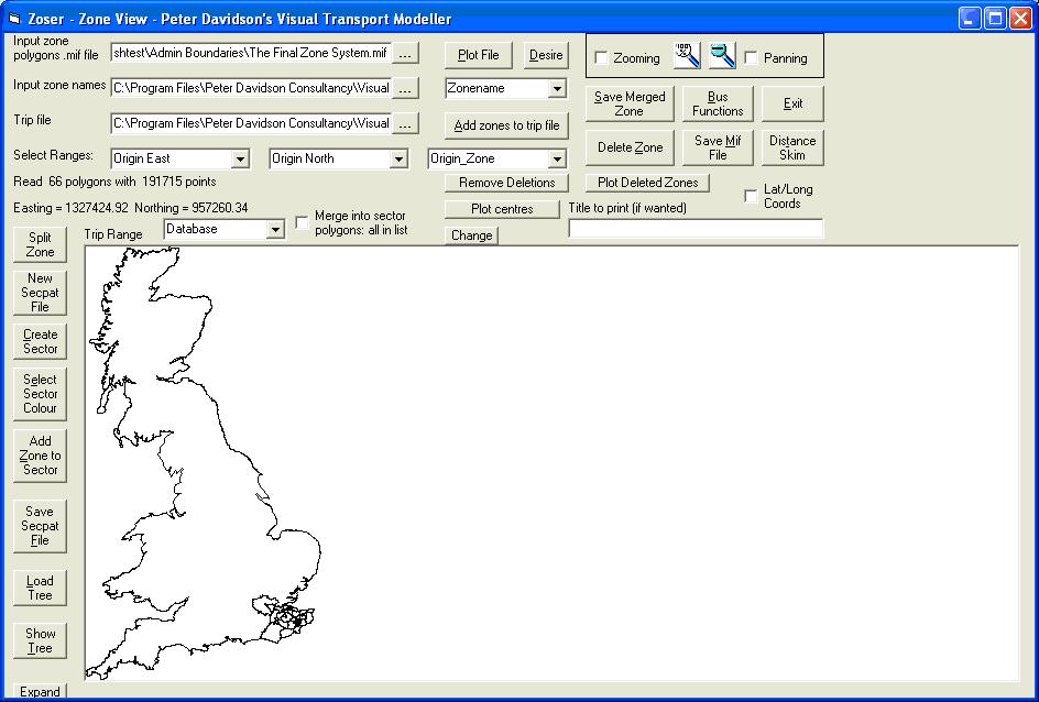
Now click Add Zones to Trip file. The Address Zone Coder will investigate each record in the trip file, plot them in the zone system, calculate the name of the zone each point is in and write this name in the appropriate column of the Tripsout.xls file. The output file is always in the same directory as the Trip file and it has the same name, only with out appended to the name. If you open this file you will see it is the same as the input file, but the Origin_Zone column now has zone numbers in it.
This process can be repeated for the destination zones.
Note the Expand button in the bottom left corner. This expands the zone display so that it fills the whole of the form.
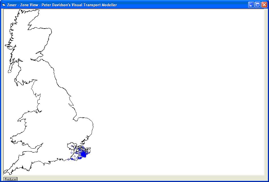
This is useful for printing screen dumps. The Expand button now has the caption Reduce and clicking it will return to the normal display.
Rezoning RSI data
Sometimes it may be necessary to rezone a set or multiple sets of RSI data. This could be the case if surveys have been carried out in several towns in a county, each using its own zone system. If at a later date it is decided to use all these data sets to build a matrix for the whole county, a unified zone system will have to be developed and the data converted to it so that the matrix can be built.
This is unlikely to be as straightforward as simply changing each zone number in the original zone systems to a number in the new one. A survey conducted in one town will probably use a detailed zone system in that town but treat each of the other towns as a single zone. The unified system may have each town divided into many zones; so one end of a trip may have to be split between many zones even though the other end is just given a new zone number. Furthermore, this splitting may require different proportions of a trip to be assigned to some of the new zones than to others, depending on their size or their population. Simply dividing a town into ten and saying that one tenth of all trips to or from that town originate in each zone may not be sufficient.
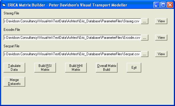
The Erica Matrix Builder provides a solution to this problem that allows a set of RSI files to be rezoned according to any desired pattern. This is called up using the Merge Datasets button on the Erica main screen.
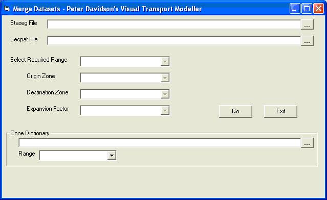
The Staseg file is selected and then the required selections are made in the drop down boxes in exactly the same manner as described in the section on RSI Matrix Building. The Secpat file that describes how to rezone the matrix is also selected. It is important to note that this is not in the same format as the secpat file that is used in matrix building, as a matrix building secpat file serves only to squeeze the zones in the RSI data down to sector numbers in the output matrix.
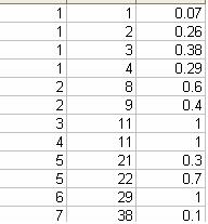
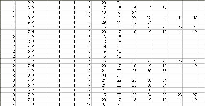
A secpat file for rezoning is in the same format as the Zonesplit file that is used to split sector cells proportionately between zone cells when expanding a matrix as described in chapter 16. This file must be in comma separated variable format with three fields on each record. These are in the form Original Zone Number, New Zone Number, Fraction. Each original zone number is repeated on as many records as there are zones between which it is to be split, followed by the number of one of the zones into which it is to be split and then the fraction (expressed as a decimal) of its trips that are to go to this zone. Using this format it is possible to assign all the trips in several sectors to just one zone by putting 1 as the fraction. It is therefore possible to squeeze some parts of the original zone system while expanding others.
This example shows zone 1 in the original zone system being split between zones 1 to 4 in the new system and zone 2 being split between zones 8 and 9 in the new system. Zones 3 and 4 are both assigned entirely to zone 11 i.e. they are being squeezed to one new zone. Zone 5 is split between zones 21 and 22 and zone 6 is assigned to zone 29 i.e. it is just renumbered.
A zone dictionary may be used, as during matrix building. Its format is described in Section 6.8.7 and it is required if the original zone numbers are non-numeric as the Zonesplit file, just like a secpat file, may only contain numeric values.
Reversing RSI data
RSI surveys are normally only carried out in one direction and it is assumed that some of the traffic (e.g. people going to work in the morning rush hour) will be reversed at a different time (e.g. the evening rush hour). If the RSI files are in Excel, ERICA can reverse them according to the users specification. The reversal will be done for the file currently named on the Staseg form.
To do this, first enter ERICA by selecting Matrix Building from the Methods menu. This opens the form below:
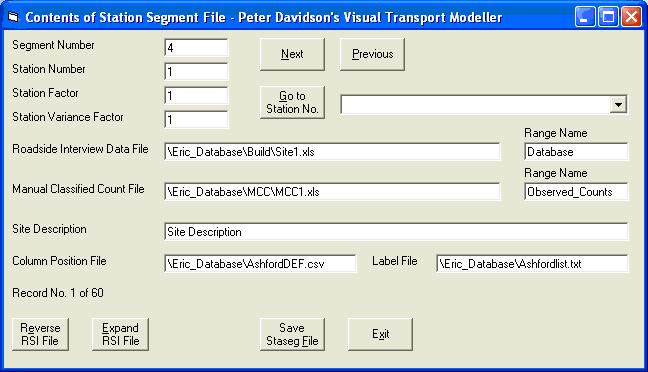
Click the top View button to open the Staseg form:
Click the Reverse RSI File button to display the reverse RSI File form:
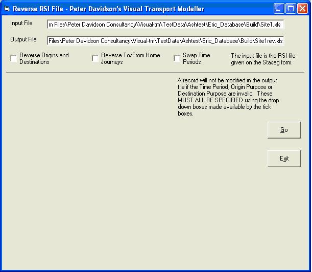
The input file is the one named on the Staseg form and the reversed output file will be in the same directory and have the same name except that it has the letters rev at the end of the name.
The check boxes allow the origins and destinations to be reversed, to and from home journeys to be reversed and up to five specified time bands to be reversed. Set all three to reveal other controls on the lower part of the form:
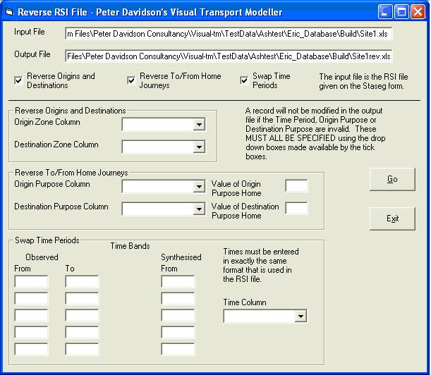
If the Reverse Origins and Destinations option is chosen, the Origin Zone Column and Destination Zone column need to be selected from their respective drop down boxes.
If the Reverse To/From Home Journeys option is chosen, the Origin Purpose Column and Destination Purpose Column need to be selected from their respective drop down boxes. The values representing Home Origin and Destination Purposes also need to be entered. They are both 1 for these files.
The time bands that are to be reversed are entered in the remaining text boxes. If the morning and evening rush hours are to be swapped, for example, enter 700 in the first Observed From text box and 1000 in the Observed To text box. Put 1500 in the Synthesised From text box. The times have to be entered in exactly the same format that is used in the RSI file. The above values will replace any time between 700 and 1000 with a time in the equivalent time band starting at 1500. 700 is therefore replaced with 1500, 730 with 1530and 930 with 1730 etc. All times therefore have 8 hours added to them, the difference between the Observed From and Synthesised From times.
For the evening rush hour, enter 1500 in the second Observed From time, 1800 in the Observed To time and 700 as the synthesised From time. This will replace all times between 1500 and 1800 with a time eight hours earlier. The Time Column needs to be selected from the drop down boc.
The form should now look like this:
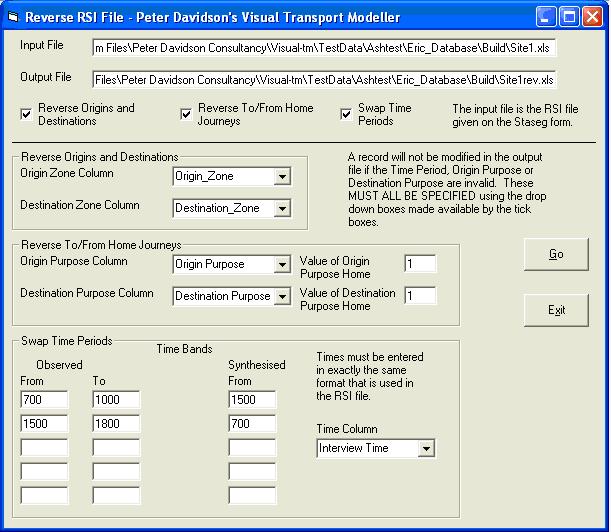
Click the Go button and the output file will be created.
RSI expansion
When Roadside Interviews (RSIs) are conducted it is likely that some kind of automated or Manual Classified Count (MCC) coincides with it. The quality data is collected during the RSI but there are obviously far more recorded journeys in the MCC, i.e. every car is counted but only a proportion are interviewed. This next stage of the tutorial will investigate the procedure for expanding RSI data to match the quantity of journeys recorded in the MCC.
Simple expansion
Open the test data and open the Staseg form as described above. Click the Expand RSI File button and the form below will open: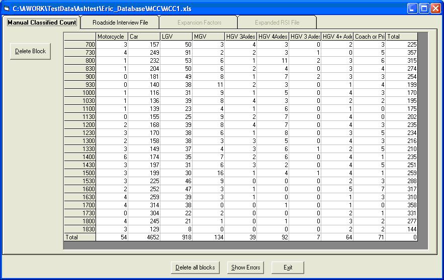
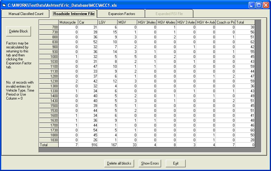
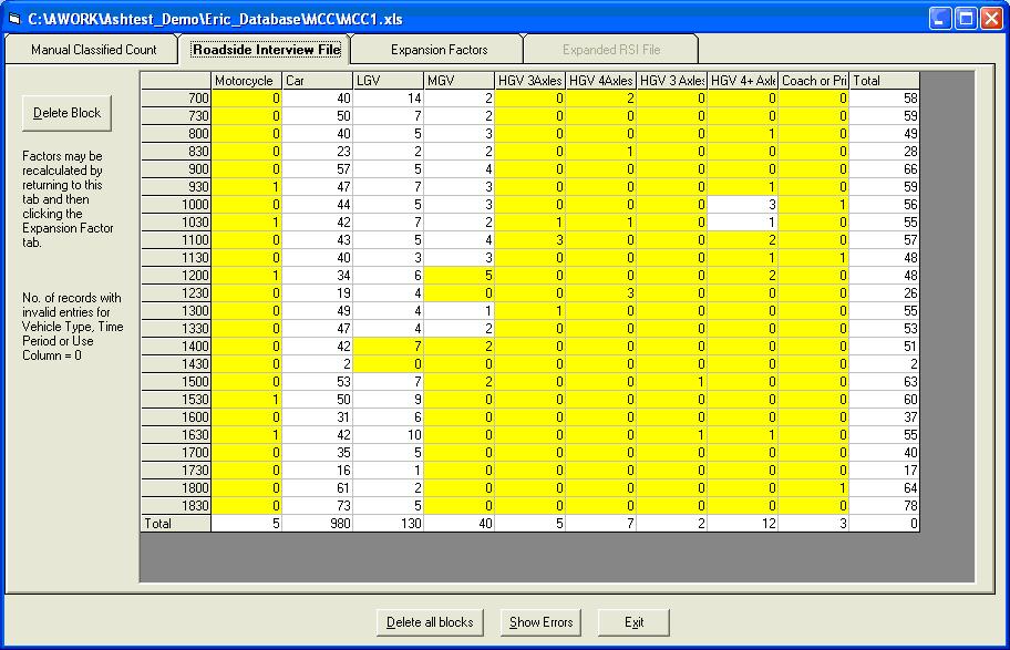
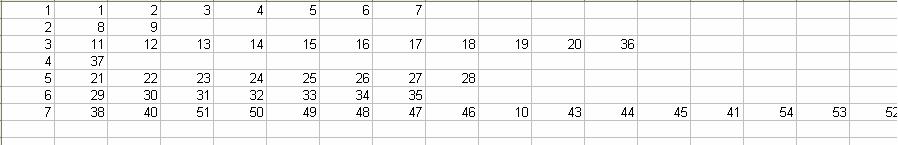
Manual Classified Count This first screen shows the raw data from the MCC file. Click the Roadside Interview File tab. This automatically displays the RSI data on the next tab screen (below)
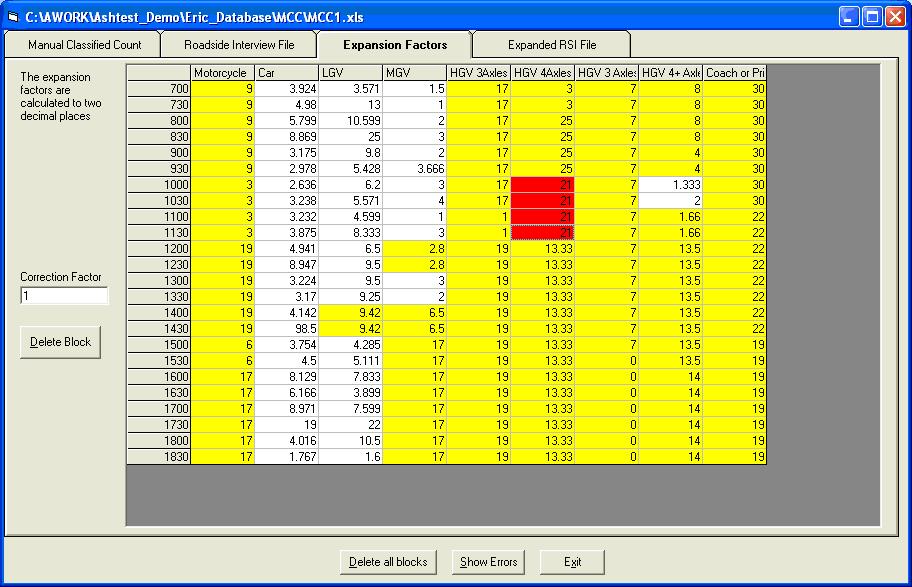
Roadside Interview File This shows the raw data from the RSI file. Click the Expansion Factors tab. Again this automatically calculates the expansion factors (below).
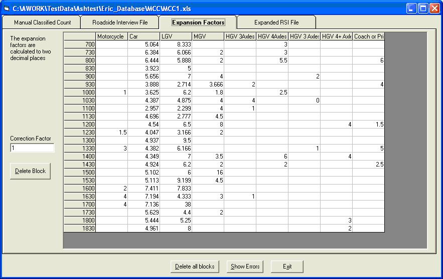
Expansion Factors You can now see the same matrix as before but with new values in the cells. These are the expansion factors, which need to be applied to the RSI file. Click the Expanded RSI File tab to add these expansion factors to your RSI file. This may take a few moments. When completed an error report screen will appear. Click OK to close.
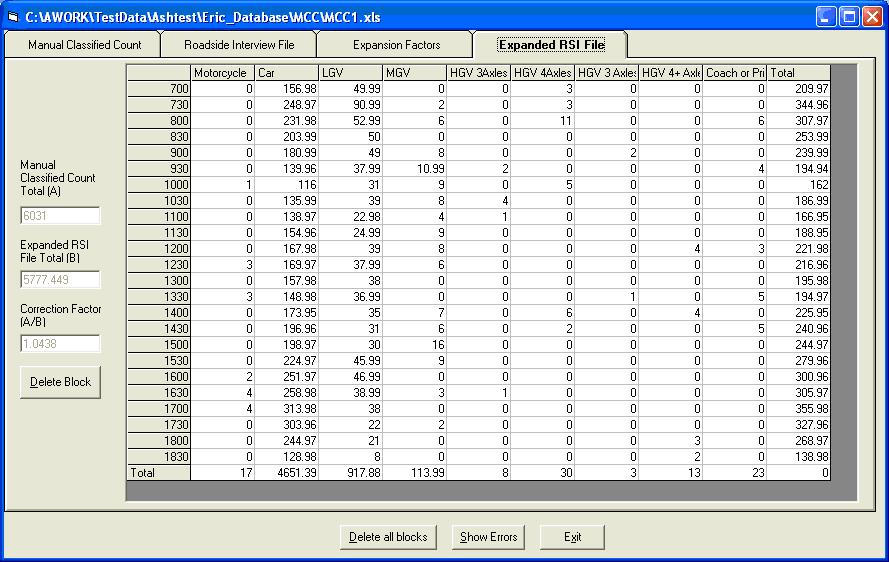
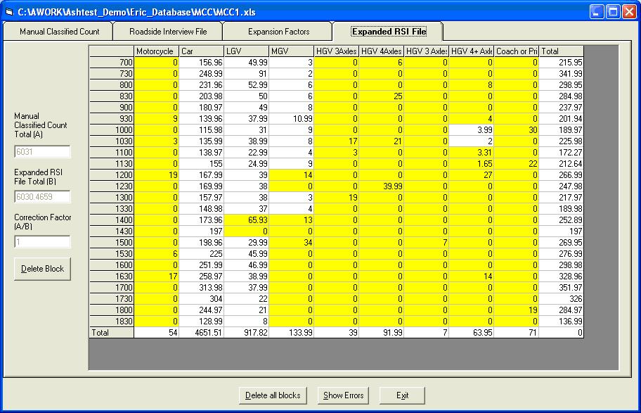
Expanded RSI File The values that are now given have had the expansion factors applied to them. On the left hand side of the screen there are three values:
Manual Classified Count Total (A) This indicates the total number of recorded instances in the MCC File Expanded RSI File Total (B) This indicates the total number of recorded instances in the Expanded RSI File Correction Factor (A/B) This shows the correction factor. This is calculated by dividing the MCC Total by the Expanded RSI total. Obviously the closer to 1 this value is the more accurate the expansion factored RSI file is likely to be. Once your RSI files have been expanded, the original file without the expansion factors will be stored with bk1 at the end of the filename.
Block definition for calculating expansion factors
At an RSI site, there will sometimes be periods when no vehicles of a particular type are stopped for interview, and sometimes no vehicles of that type will be recorded by the MCC count. This means that some expansion factors cannot be calculated and means that when the RSI file is factored up by the expansion factors, the results will not be equivalent to the MCC file.A solution to this problem is to group time periods and/or vehicle types so that all zeroes are averaged out with neighbouring non-zero cells. This is done by defining blocks on the grid, so that all MCC observations in a block are divided by all RSI observations in the block to give an averaged expansion factor that is applied to all individual cells in the block. It is recommended that the blocks are single column so that time periods are grouped and not vehicle types. This ensures that the vehicle type totals remain the same in the MCC file and the factored up RSI file.
Open the test data as described above and click Next on the Staseg form to display the details for Site3.xls. Click Expand RSI File. The result should be as follows:
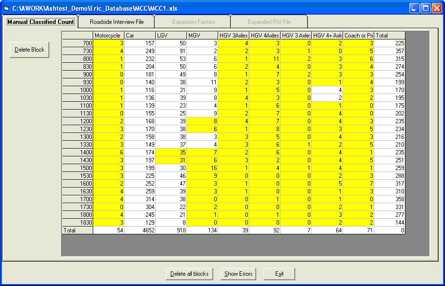
All cells that have been grouped in a block have a yellow background. This is only observed if the file specified on the Staseg form is Site3.xls as the test data does not have files giving block patterns for the other files. A block file belongs in the same directory as the RSI file and has the same name, only with block at the end of the name and a txt extension. Erica checks if the file exists when it opens the MCC file and if it does, it displays the block pattern.
Clicking on the other tabs will show the same pattern. The blocks are all within individual columns and it is possible to identify the block that any cell is in by clicking on it. This displays the block in question in red. Click the Roadside Interview tab and then the Expansion Factors tab to calculate the factors.
Note that within a block the expansion factors are all the same e.g. HGV 4 Axles from 1000 to 1200, selected above by clicking one of its cells.
Click to display the Expanded RSI file and to save the factors to the RSI file. Note that the correction factor is 1 and the totals for each vehicle type are within 0.5 of the values in the MCC file, indicating that all zeroes have been grouped and that all groups are within a single column.
Defining Blocks
Click Next again on the Staseg form and expand the RSI file for Site5.xls. It will be displayed without blocks, as there is no block file for the Site5.xls RSI file. To define a block, click on the top left cell that is to be included and drag to the bottom right cell. In a single column block, just click the top cell and drag to the bottom one. To group motorcycles from 700 to 900, click 700 and drag down to 900 before releasing. The block will be highlighted in red.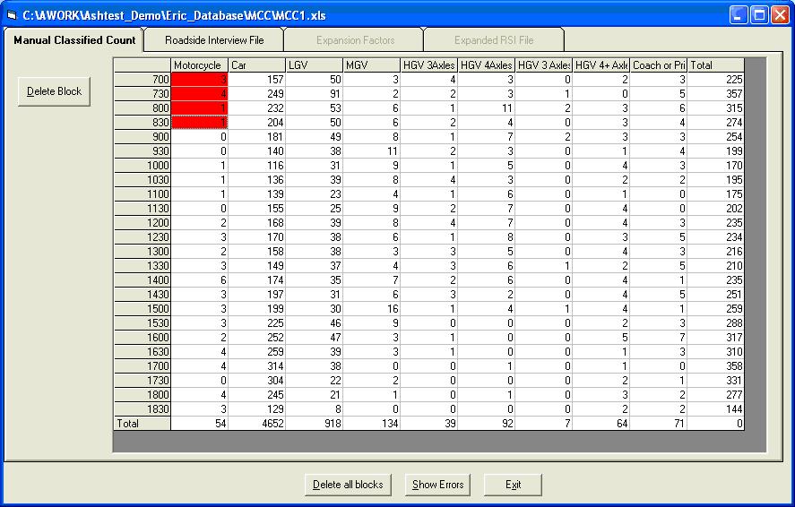
Repeat for motorcycles from 900 to 1130.
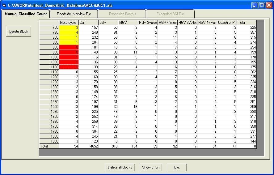
The first block goes yellow and the latest one is coloured red. This will be repeated as the block pattern is defined. The blocks may be defined on any of the four tabs so all of the data that the form displays can be use to help define them. The block structure is saved whenever a tab is clicked or the form is closed using the Exit button or the cross in the right hand corner.
The complete block structure can be deleted at any time by using the Delete all Blocks button. This returns all the grids to a white background and deletes the file with the block pattern. Any individual block may be removed by clicking it, followed by the Delete Block button. This will always remove the block displayed in red.
Market segmentation in your excel data
If a field is required for market segmentation, there must be a range with the same name as the field in the first data file listed in the Staseg file. This range must have the same name as the field and should give the name of each value that the field can have, listed in numerical order in the first column of the range.
In the test data the first data file listed in the Staseg file is Eric_Database\Build\Site1.xls. Open this file and you will find a number of named ranges. One of these is called Time_Period:
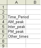
Note that there are four entries below the header in this named range. Returning to the data in this file, notice that in the Time_Period column every trip has a number between 1 and 4 (the same is true of every RSI file listed in the Staseg file). A 1 in this column indicates that this trip took place in the AM peak, a 2 indicates an inter-peak trip, a 3 a PM peak trip and a 4 a trip from any other time.
If the time period is used in a matrix build with market segmentation, then the entry in the Time_Period column determines which market segment (time period) the trip appears in.
The parameter files
ERICA uses five parameter files:
Staseg.csv
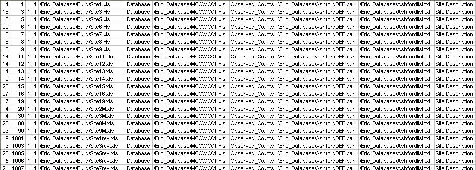
This file describes the relationship between stations and segments and is the main element of the database. It lists each of the stations in the database, one station to one line, recording which segment that station belongs to and other information such as station specific expansion factors and variances.All the roadside interview data files are called up by this file in which all the segment, station and parameter file details are listed. This is a comma separated variable file with data in the following format:
Column no. Contents 1 Segment number 2 Station number 3 Station factor 4 Station variance factor 5 RSI data filename 6 Range containing data in RSI data file 7 MCC filename 8 Range containing data in MCC file 9 Column position file 10 Label file 11 Site description Example:
Station factor
Station factors (column 3 of the staseg.csv file) simply multiply each trip record expansion factor in that RSI file by the factor given. This may represent a growth factor to present year. These can be input as a given factor or as 1.Station variance factor
RSI sites can be given a variance expansion factor (column 4 of the staseg.csv file), for example if a sites transpose is being used it will be less accurate than the original direction, so should be given a higher variance. Again, this can be input as a given factor or as 1.Secpat.csv
This file describes the relationship between zones and sectors. It lists out the sectors used in the study together with the zones contained within each sector. Sector and zone numbers are acceptable up to a maximum of five digits. Sector numbers are entered in the first column; zone numbers are then listed in the following columns. Hyphens can be used to group consecutive zones, e.g. 1-4 for zones 1, 2, 3 and 4.Example:
Ercodm.csv
This file records the segments selected from which to extract data for each sector-to-sector movement for input into the trip matrix. Since the segments are arranged into cordons, this is commonly known as the cordon file. For each sector to sector movement up to six cordons may be selected and ERICA calculates a weighted average for input into the trip matrix. Section 6.c of the separate ERICA5 manual sets down the rules for cordon selection and is the product of knowledge built-up during the ERTM and SERTM studies.For each sector-to-sector movement defined there is at least one cordon specified. The file format is given below. Each cordon should form a complete barrier around one of the specified sectors.
Column no. Contents 1 Origin sector 2 Destination sector 3 Positive or negative 4 Cordon no. 5 Factor 6 onwards Screenline segments which make up the cordon for this sector to sector movement Care should be taken when entering sector numbers in that they must correspond to those given in the Staseg.csv file. For example if sector 0001 is specified in the ERICA cordon file then it should be referred to as this in all cases and not reduced to 1 or 001 etc.
Example:
Column position file
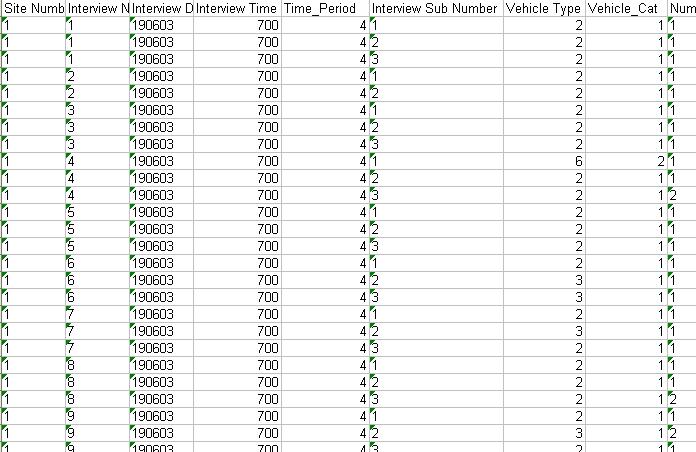
The RSI definition file, in this case AshfordDEF.csv defines the layout of the RSI data, giving the positions of the important fields that are required for matrix building.Example:
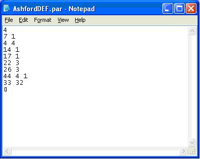
The number on the first row is not used, but must be present to maintain the correct file format. The first numbers on rows two to seven give the positions of required columns in the Excel files as follows:
Row 2 Vehicle Type
Row 3 Time Band
Row 4 Origin Purpose
Row 5 Destination Purpose
Row 6 Origin Zone
Row 7 Destination Zone
The second numbers in these columns gave the field widths for data held in fixed width text files and are therefore irrelevant here as we are using spreadsheets, but there needs to be a digit present to maintain the file format. Rows 4 to 7 are used for transposing the file (see Section 6.5.7.1.), but not when calculating the expansion factors.
Row 8 must have three numbers on it, of which the first two are not used and the third is called the Unit of Expansion. This is more likely to be of use with text files where it allows expansion factors to be written without decimal points e.g. an expansion factor of 9.74 could be written in a text file as 974 and a Unit of Expansion of 100 would tell the software to divide by 100 to obtain the correct value. The Unit of Expansion is set to 1 for this data.
The final gives the Expansion Factor column followed by the Use Record column. The Expansion Factor column should be a blank column in which the expansion factors will be written once they have been calculated.
The Use Record column is a flag that says whether a record should be taken into consideration when calculating the expansion factors. A record may be rejected due to invalid or missing data in a field or if there is some other problem regarding its accuracy. A number 1 should be entered in the field if it is to be used and a zero if it is to be ignored. If the field is blank, it will again be ignored. If any other number is entered in the field, the record will be taken to consist of this number of trips e.g. a value of 1.25 in this field will cause the record to be treated as 1.25 trips instead of one trip.
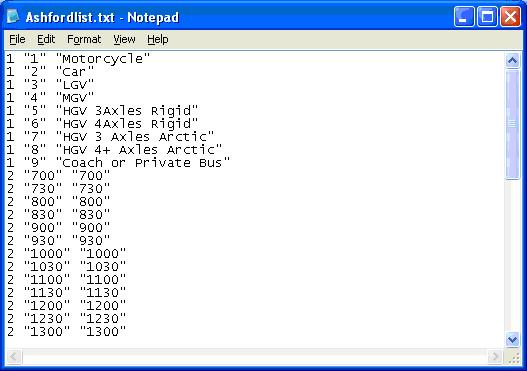
Label file
This file is needed for expanding RSI files, but not for matrix building. It defines the Vehicle Types, Time Periods, Origin Purposes and Destination purposes that are used in the RSI and MCC data. They have to be listed in that order and the value in the first column says what category each row belongs to i.e. 1 signifies a Vehicle Type, 2 a Time Period, 3 an Origin Purpose and 4 a Destination Purpose.The second column is the value that appears in the field in the RSI and MCC files and the third column is its description. This is the text that labels the rows and columns on the grids when the RSI files are expanded.
Example:
RSI matrix building
ERICA is entered by selecting Matrix Building from the Methods menu. This opens the form below:
Click on the Build RSI Matrix button to open the following form:
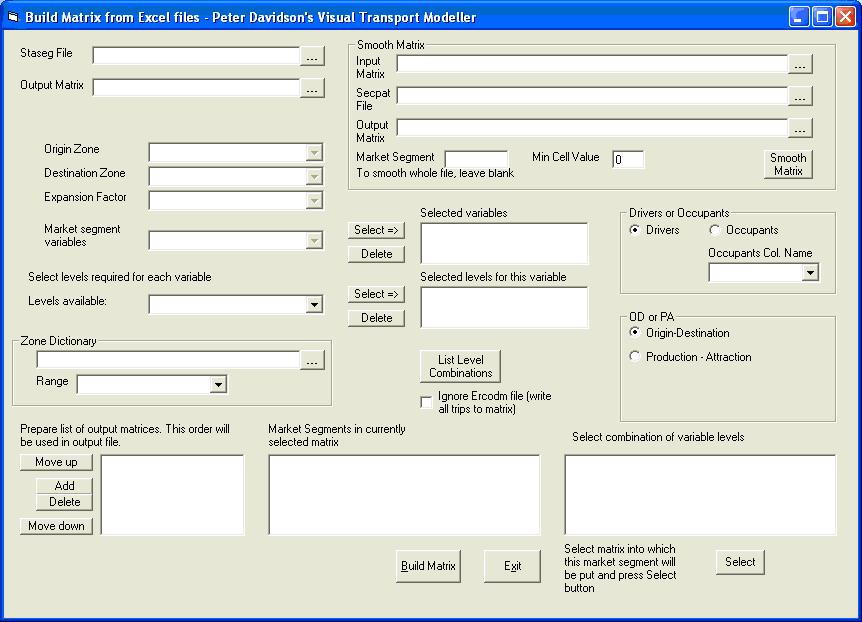
Browse to the staseg file and open it. Use the browse button next to the Output Matrix box to choose a name and location for your output matrix. Select the the range which contains all the data in your RSI files in the Select Required Range drop down box. For the test data this range is called Database.
Next select the columns which contain the origin and destination zones and the expansion factors from their respective drop down boxes. For the test data these are Origin_Zone, Destination_Zone and TotalExpansionFactor. The form should now look like this:
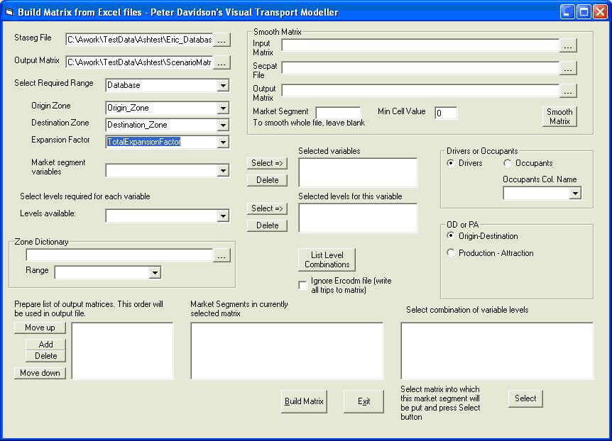
Click Build Matrix. A message will appear at the bottom of the form displaying the progress of the matrix build. When it is completed the message will display the number of input and output trips and how many records could not be processed due to invalid data.
Matrix building with market segmentation
If a field is required for market segmentation, there must be a range with the same name as the field in the first data file listed in the staseg file. This range must have the same name as the field and should give the name of each value that the field can have, listed in numerical order in the first column of the range. See the example in the test data and the more detailed explanation in the market segmentation section of this chapter.On selecting the field in the Market segment variables box, these names will be listed in the Levels available combo box. If the necessary range does not exist, a message will be displayed. Select one of the required levels and click the Select button next to it to add it to the Selected levels list. It can be removed using the Delete button if it was added by mistake. Select the rest of the levels required for this variable and when they have all been chosen, select the next variable required from the Market Segment variables combo box and proceed as before.
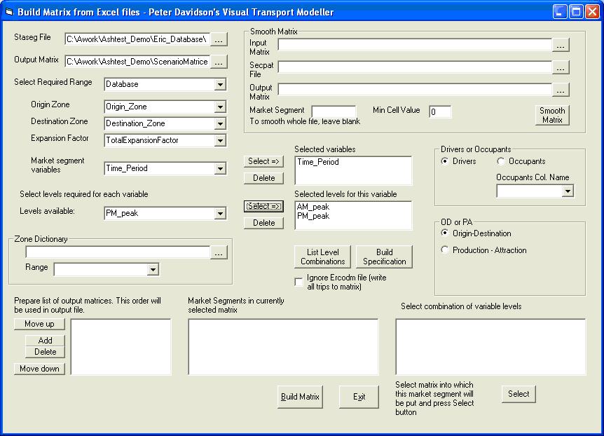
Using the test data as an example, fill in the Build RSI Matrix form as described above. Now select Time_Period in the Market segment variables drop down box, click Select and then choose AM_peak in the Levels drop down box and click its Select button. Then choose PM_peak and Select. The form should look like this:
Now select Vehicle_Cat from the variables drop down box, click Select and then choose Car, MC, LGV from the Levels available list followed by HGV.
When all the required variables and their levels have been chosen, click the List Level Combinations button. This will list all possible combinations of the selected variable levels on the list headed Select combinations of variable levels. The required combinations can now be linked to Market Segment numbers in the output Binary ERICA matrix. To do this, click the Add button and enter a name for the first market segment. Select it in the list and then select the combination of variable levels in the list that is to be written into it and click the Select button below the list. If any other combinations of levels are to be added into it, select them in the list one at a time and click the Select button. Any number of combinations may be added together in a market segment.
When all choices have been made for a market segment, click the Add button and enter a name for the next market segment. Proceed as before until all market segments have been created. Unwanted market segments may be deleted and the order of the market segments may be changed using the Move up and Move down buttons. The final order will be used in the output matrix.
Continuing the above example, after clicking List Level Combinations add a matrix called AM and then select AM_peak Car,MC,LGV from the combinations list and click Select. Then click on HGV and click Select. Now add a matrix called PM light and select PM_peak Car,MC,LGV. Add a third matrix called PM heavy and select HGV. The form should now look like this:
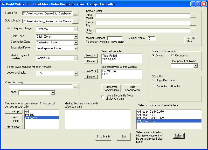
Selecting any matrix already on the list e.g. AM will list the combinations in it in the box headed Market Segments in Currently Selected Matrix
Matrices can be built using vehicle occupancy to give the total number of people travelling instead of the number of vehicles. To do this, click the Occupants option and use the combo box below it to select the column giving the number of vehicle occupants.
When everything has been set up, click the Build Matrix button. The output matrix will have three market segments, with the first having the trips made in the AM peak. The second has the PM peak trips made by car, motorcycle and LGV. The third has the PM peak trips made by HGV.
RSI matrix outputs
Two files are produced in a matrix build. The one with the name specified by the user is the positive matrix. The one with neg at the end of the filename is the negative matrix. To get the total matrix simply subtract the negative matrix from the positive one using Visual-tms Matrix Calculator.
Other data matrix building
To build a matrix from household interview data, choose Build HHI Matrix on the main Erica form. The form below will open:
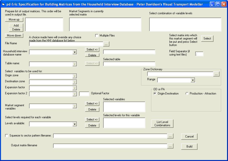
In the File Name box browse to the location of your HHI data file. Select the range which contains all the data in the Table name drop down box, and click the select button to the right of this. As with the RSI build, choose the columns containing the origin and destination zones and the expansion factor in their respective drop down boxes. Finally use the browse button next to the Output matrix filename box to choose a name and location for your output matrix. The form should now look like this:
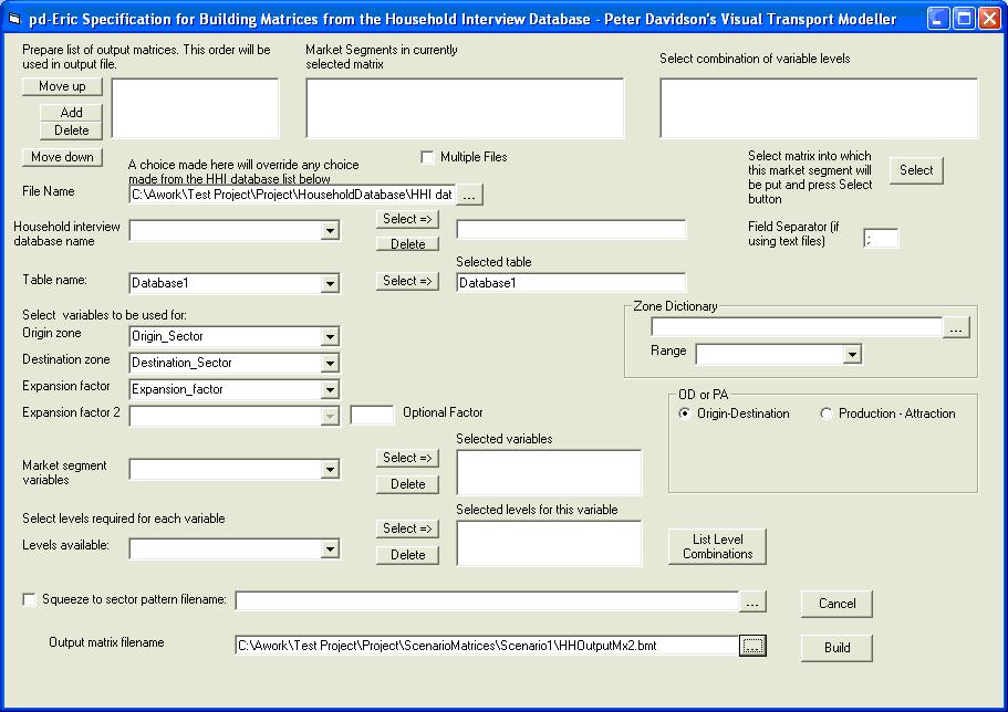
Click Build. A message will appear at the bottom of the form displaying the progress of the matrix build. When it is completed the message will display the number of records read and how many could not be processed due to invalid data.
Overall build specification
Matrices can be built from one data source with a market segment variable inferred from another data source.
For example, RSI surveys do not contain data about car availability for car passengers. Household interview surveys do contain this information, but there are fewer of them. It is possible to take the data from the HHIs and use it to infer car availability for an RSI matrix build.
In order to do this a spreadsheet file called OverallBuildSpec is needed. See the example in the test data.
With the test data loaded, click the Overall Matrix Build button on the main ERICA form. This will open the form below:
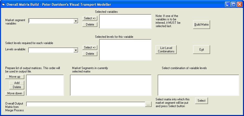
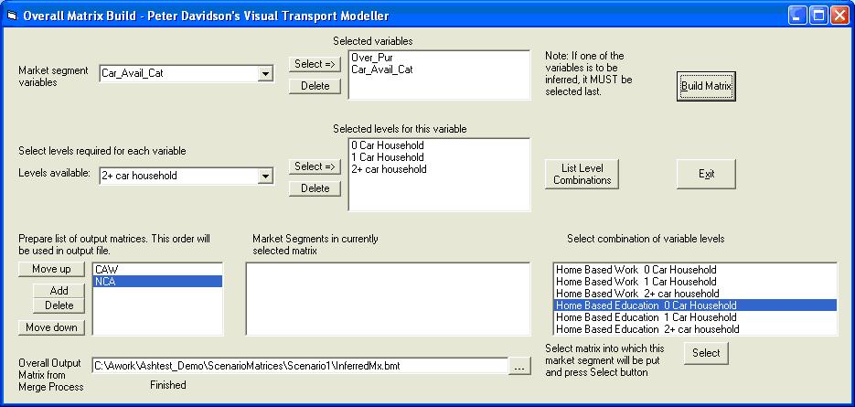
In the same way as on the matrix building screen, select the market segment variables and levels you want in your matrix. The variable to be inferred must be selected last. For this example choose Over_Pur with the levels Home based work and home based education. For the variable to be inferred choose Car_Available_Cat and the levels 0, 1 and 2+ cars available. Create two market segments, one with home based work 1 car available and home based work 2+ cars available, and the second with home based work 0 cars available and home based education 0 cars available. Choose an output matrix name and click Build Matrix. A message will be displayed when the process is finished:
Back to tutorials On to assignment models