![]()
![]()
![]()
![]()
![]()
![]()
![]()
![]()
Back to tutorials On to mode choice models Covered in this section:
- Description
- Requirements
- The assignment form
- Highway assignment options
- Public transport assignment options
- Combined mode assignment options
- Outputs from the model
- Viewing on the network
- Assignments between specified O-D pairs from matrix editor
- Skimming, best path etc.
Description
Assignment modelling is the procedure for allocating trips in a matrix to the simulated network in order to predict traffic flows over links. The methodologies for creating and manipulating trip matrices and networks are covered in detail in the tutorials on matrices, matrix building and networks.
Requirements
The first stage when conducting an assignment model is to ensure the required scenario network is currently built. Use the Dataviewer to build the Base and Scenario1 network, i.e. the do nothing scenario. Lets conduct the base assignment.
The Assignment form
Click Models/Assignment to open the Assignment form:
Highway assignment options
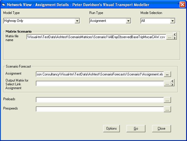
We will now demonstrate the procedure for undertaking a highway assignment model run. First open the Ashtest project, then open the Assignment form as described above.
Select Highway Only from the Model Type drop down menu and Assignment from the Run Type drop down menu. The Mode Selection drop down menu can be used to bias the assignment towards a particular mode (described later). For now leave it set to All.
Under Matrix Scenario/Matrix file name click
and browse to the matrix to be assigned. For this example we are using AllDayObservedBaseTripMxcarCAW.csv saved under Scenario Matrices\Scenario1. Select it and click Open.
The matrix to be assigned has to be in either binary ERICA, comma separated variable or O-D cell format. If you choose a binary ERICA matrix for assignment you must also select the market segment and whether to use records, trips or variances from it. If the matrix to be assigned is a comma separated variable or O-D cell matrix, these drop down boxes and their labels on the Assignment form become invisible as they are not needed.
The scenario forecast assignment file is one of the output files from the assignment model run. It is useful to store these files relative to the network and matrix scenario that they relate to. Click
If you wish to preload flows for an assignment, a previously produced pbAss.dat should be selected in the Preloads text box. If you wish to preload speeds, it should be entered as the Prespeeds file. This file will be explained in more detail later. For now these two boxes can be left empty.
The form should now look like this:
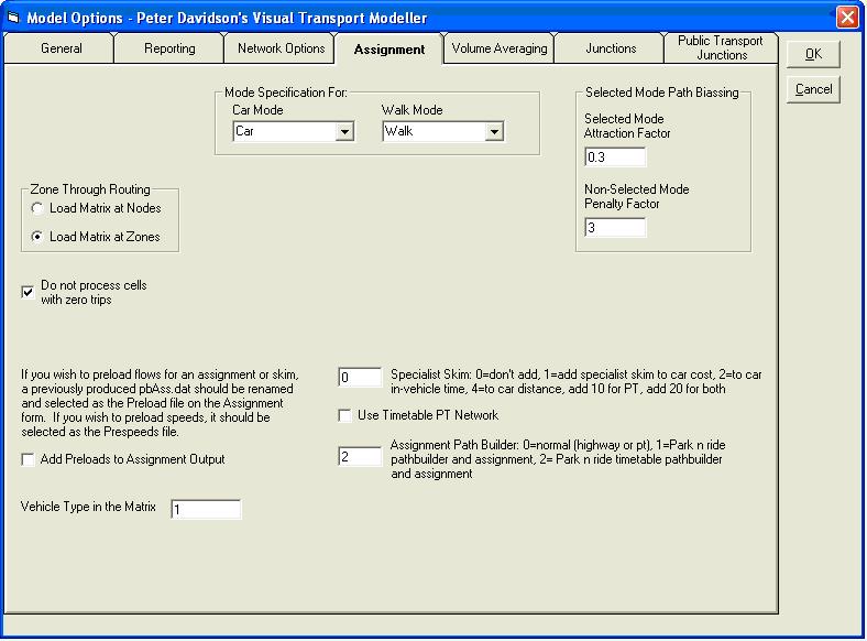
Next click the Options button. This calls up the Model Options form, which is already set up for the Ashtest project. The main important things to check are that the number of zones is set correctly on the General tab, and the Car and Walk modes are set on the Assignment tab. Click OK to return to the Assignment form.
Click Go to run the assignment model.
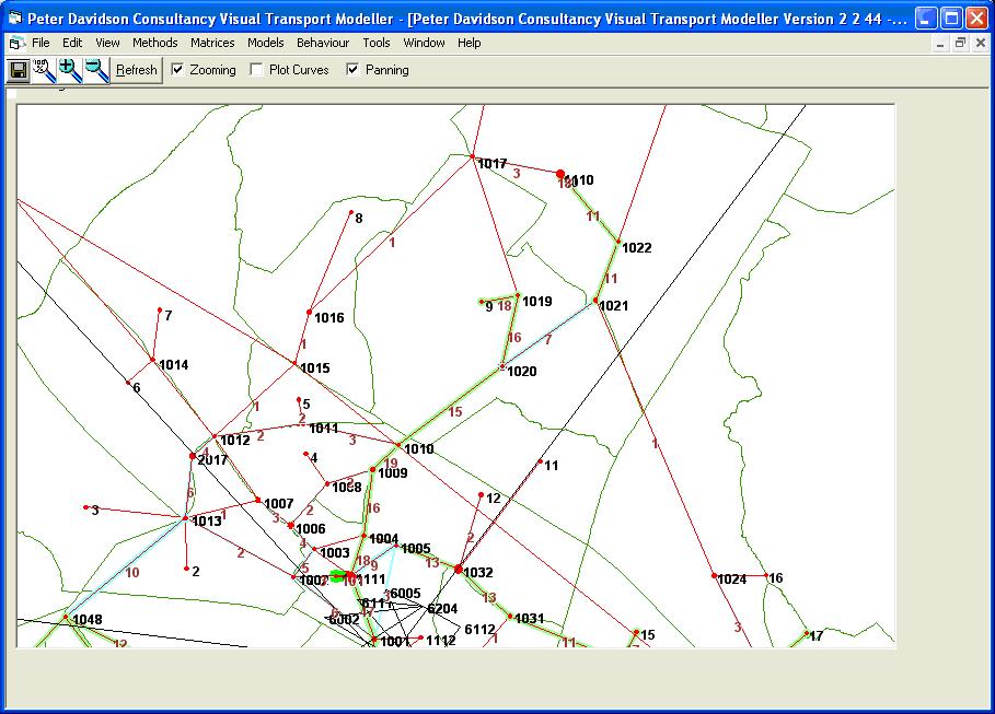
Once completed, the Assignment Details form will close and the trips are plotted on the network. You may need to zoom in to view them (below):
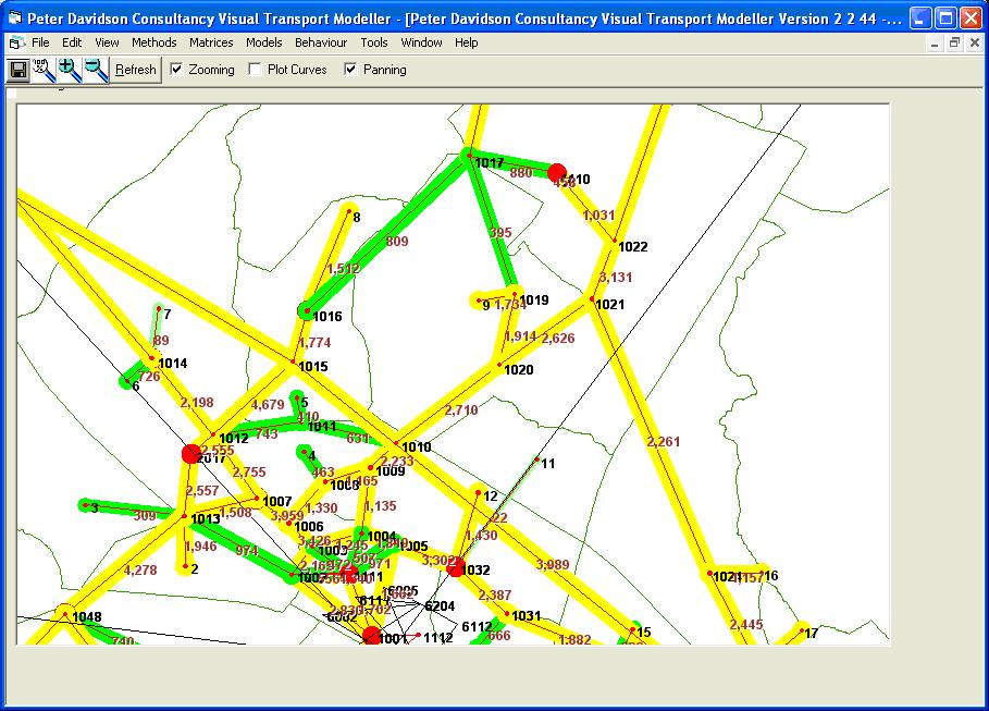
Model outputs and viewing flows on the network are described fully in later sections of this tutorial.
Highway assignment with junction delay
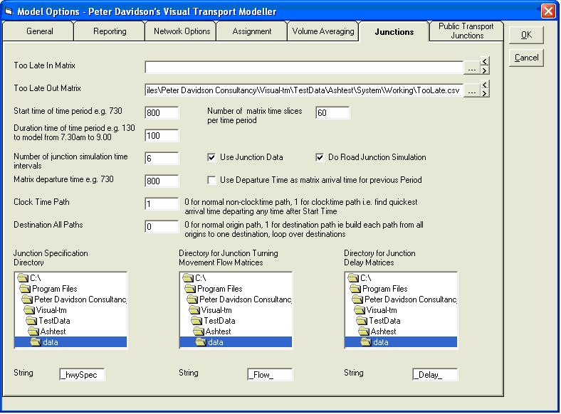
If the network has been coded with highway junctions as described in the networks tutorial then a highway assignment can be run with junction delay. Set up the Assignment form in exactly the same way as described above. Click the Options button to open the Model Options form and then go to the Junctions tab: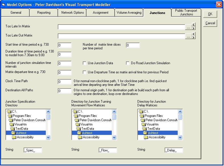
The Use Junction Data and Do Road Junction Simulation boxes should be ticked. The directory containing the junction specification files should be selected under Junction Specification Directory and the entry in the box labelled String under this should read _hwySpec. The rest of the form should be set up as follows (for an explanation of what all the entries are for please refer to chapter 26 of the Visual-tm manual):
On the Assignment tab 2 needs to be entered in the Assignment Path Builder box and 1 in the Vehicle Type in the Matrix box:
Click OK to close the form then Go to run the matrix. The usual assignment model outputs will be produced as well as flow and delay matrices for each junction. These will be created in the location specified on the Junctions tab of the Model Options form.
Public transport assignment options
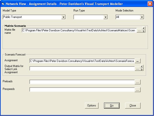
To run a public transport assignment, the Assignment form should be set up in the same way as for a highway assignment, except that Public Transport should be chosen as the Model Type instead of Highway Only.
Click the Options button to go to the Model Options form. For public transport assignments, a choice is made between one reference path and multiple reference paths. One reference path will assign all the trips to the most frequent route between two points and multiple reference paths will split them between routes according to the headways. The default is to use one reference path. The tick box marked Allow Walking on Public Transport Links should normally be left ticked, which is its default setting. If it is not ticked, people will not be allowed to walk along the links used by public transport routes.
Click Go on the Assignment form to produce the following. The matrix assigned here is ScenarioMatrices\Scenario1\AllDayObservedBaseTripMxPtCAW.csv:
Combined mode assignment options
There is no park and ride data in the base network, however, scenario 6 does contain park and ride data. Use the Dataviewer to load this scenario and then open the Assignment form.
To do a Park and Ride assignment, choose Park and Ride, Public Transport and Highway as the Model Type on the Assignment form. The rest of the form is set up in the same way as before.
Click the Options button to go to the Model Options form. You will notice there are some extra Park And Ride options on the Assignment tab:
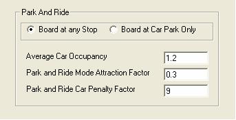
The Board at any Stop/Board at Car Park Only option specifies where in the model people can change mode from their car to the park and ride bus either anywhere on the bus route or at the car park only. The average car occupancy, mode attraction factor and car penalty factor are also set here.
Click Go on the Assignment form to run. The flows shown on the display are the public transport part of the assignment. The car part can also be plotted as described in the Viewing on the network section below.
Outputs from the model
Outputs from a highway assignment
The two main outputs from a highway assignment are Assignment.xls and pbAss.dat.Assignment.xls is the scenario forecast assignment file specified on the Assignment form. An example is shown below:
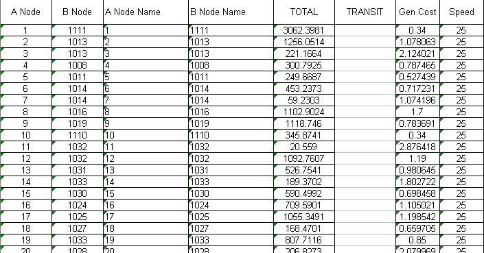
Each row corresponds to a link in the network. The first two columns give the A node and B node numbers of the link. The next two columns give the names of these nodes. The TOTAL column contains the number of vehicles travelling on the link. The Gen Cost column contains the generalised cost of travelling along the link, and the Speed column gives the speed on the link.
PbAss.dat contains much of the same data. It is output in the projects System\Working directory. An example is shown below:
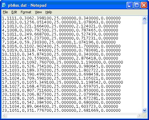
Again, each row corresponds to a link in the network. The first two columns give the A node and B node numbers of the link. The third column is full of zeros. The next three columns are the flow, speed and generalised cost; and the final column is also full of zeros.
If for a later assignment or skim you want to use the flows or speeds from this assignment, then this pbAss.dat file is entered into the Preloads or Prespeeds filename box on the Assignment form.
Outputs from a public transport assignment
Public transport assignments output an Assignment.xls file exactly like highway assignments. The flows shown are the totals on the links, but these are broken down to show how many trips are being made on each route that uses the link in a file called PTAssignment.xls. This is in the same directory as the Assignment.xls file specified on the Assignment form. This has the same format as the Assignment.xls file except that each link is repeated for each route that uses it so the flows refer to each route and not to the total on the link. The route number is given in column F. A zero in this column indicates that no route is being used, i.e. the flow is for people walking along the link: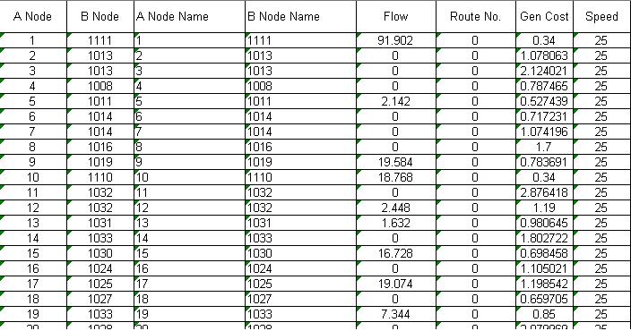
A public transport assignment also produces a pbAss.dat file in the projects System\Working directory. This contains the same data as a highway pbAss.dat, but now the third column contains the route number instead of just zeros.
Another file produced is called RouteReport.dat, which will also be in the System\Working directory:
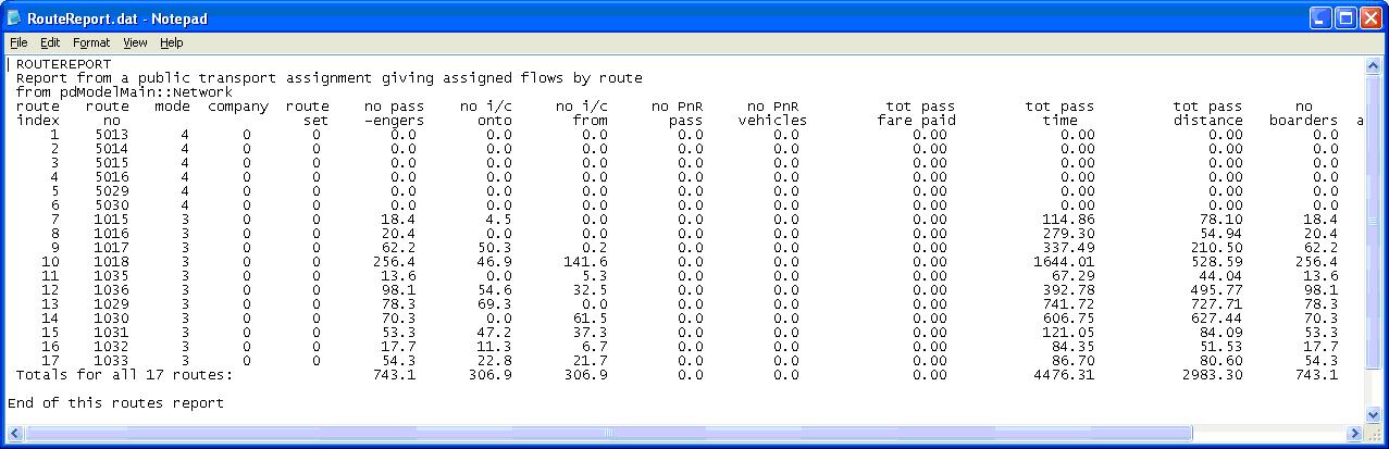
This report contains useful information about each route, such as the total number of passengers and the total fare paid.
Outputs from a park and ride assignment
Park and ride assignments produce the same outputs as normal public transport assignments, but in addition they produce a spreadsheet called PnRHWayAssignment.xls in the same directory as the Assignment.xls and PTAssignment.xls files. This gives the flows for people driving to the car parks to use the park and ride service.In the System\Working directory, pbAss.dat contains data from the public transport part of the assignment and HwyAssignm.dat contains data from the car part.
Viewing on the network
When an assignment is run, the Assignment form closes and the flows are displayed on the network. You may need to zoom in to view them:
On the Assignment Bandwidths tab of the Display Options form, it is possible to change the colour and width of the lines representing different flows. For this example, it is set up as shown below.
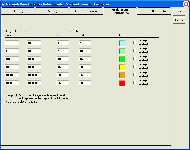
The bandwidth of the links indicates the number of trips along that link. The thicker the line, the more trips there are. The flows in each direction may be displayed separately by ticking the Plot Each Direction Separately box on the Plotting tab of the Display Options form.
To view a previously conducted assignment run Click View/Flows the form below opens:
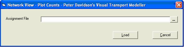
Click
Assignments between specified O-D pairs from matrix editor
There may be occasions when you wish to perform an assignment for limited numbers of O-D pairs in a larger matrix and not for the entire matrix. This may be to reduce run time or to reduce the amount of data to be displayed and analysed. This can be done by opening and displaying the matrix in the Matrix Editor and will therefore work for any matrix format that this is capable of reading.
Ensure that the Number of Zones on the Options form is set to the total number of zones in the network. If the O-D pairs are in a single rectangular block on the grid, just select this rectangle and on the Matrix Editor Tools menu click Do Assignment. The results will be plotted on the network. If you need to select several blocks on the matrix, click Select Multiple Blocks on the Matrix Editor Tools menu before selecting the required blocks on the grid. After selecting them all, click Do Assignment on the Tools Menu.
Skimming, best path etc.
In the Run Type drop down menu on the Assignment form there are a number of options other than Assignment. The first of these is Best Path.
Best Path
Path building is a very important aspect of Visual Transport Modeller. As in the real world there are likely to be a multitude of different routes available to the traveller moving from point A to B. The object is to find the Shortest Path available. Shortest does not necessarily mean shortest distance. As described earlier in this tutorial, each link in the network has been allocated a generalised cost. This figure could simply be the distance or the time taken to travel along the link. Alternatively it could be a complex equation, which attempts to include many variables. The level of detail included when calculating generalised costs is usually a matter of preference, budget and processing restrictions.The definition of the Shortest Path in Visual-tm is the path between two points that has the lowest cumulative generalised cost i.e. the generalised costs for every link in the path is added together and the path with the lowest total is the shortest path.
If Best Path is chosen as the run type then the software will calculate the shortest path (i.e. the path with the lowest cumulative generalised cost) between every O-D pair in the input matrix. The output is a file called pbPath.dat which is created in the projects System\Working directory:
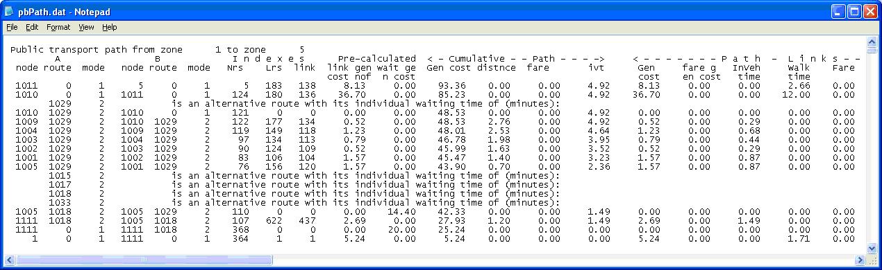
Each link in the best path is listed along with its attributes.
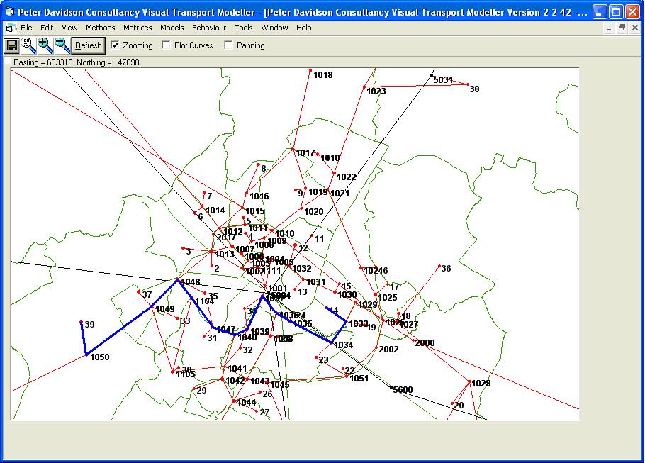
There is also a graphical method for calculating the best path. Click Methods/Shortest Path. You are now prompted to click on a node (zone centroid) in the network that will be the origin of your journey (below).
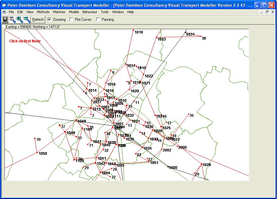
You may need to zoom into the network in order to click on a node. Once you have successfully selected the first node you will be prompted to select the second node that will be used as the destination. You can zoom in or out and pan across the network until you have successfully selected the destination node. Once this has been selected, the system will now draw the shortest path between the 2 selected points as a blue line:
To remove the shortest path from the display, right click anywhere on the network with the Panning option unchecked.
Skimming
A skim is a matrix containing a variable value for each zone to zone movement in the study area.To calculate a skim, select Skim from the Run Type drop down menu. Select the attribute you want to skim for (e.g. Length km) and enter an input matrix. It doesnt matter what is in the input matrix every O-D pair will be skimmed for. Enter Preloads and Prespeeds files if required, and enter a name for the output skim file. If this is left blank the default of System\Working\pbSkim.dat will be used.
The form should be set up like this:
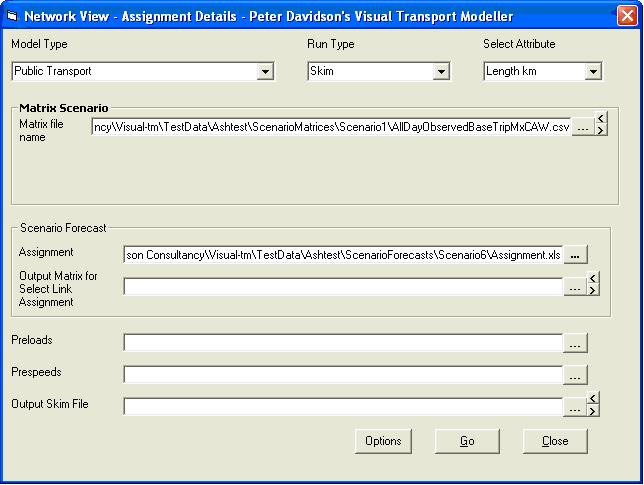
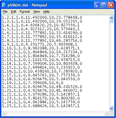
The output file is in comma separated variable format and for the above skim looks like this:
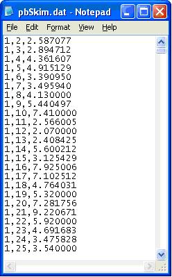
The first column is the origin zone, the second is the destination zone and the third is the length of the journey between them in kilometres.
Standard Set of Skims
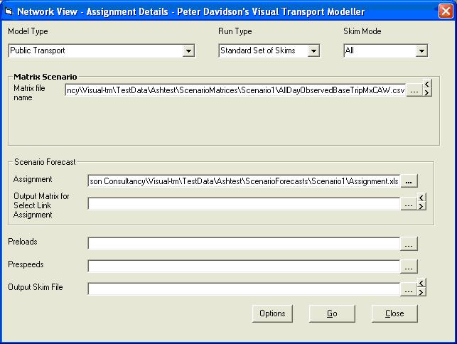
Visual-tm has been pre-programmed to produce a standard set of skims.Select the Model Type i.e. Highway Only, Public Transport or Park and Ride, Public Transport and Highway. Then in Run Type select Standard Set of Skims. A text box labelled Output Skim File is now available at the bottom of the form. You can enter a name for the output skim file here. If no name is entered, the skim file will be called pbSkim.dat and will be in the projects \System\Working directory.
Enter an input matrix. It doesnt matter what is in the input matrix every O-D pair will be skimmed for.
If you wish to preload flows for an assignment or skim, a previously produced pbAss.dat should be selected in the Preloads text box. If you wish to preload speeds, it should be entered as the Prespeeds File. For this example, we are not using preloads.
The completed form for a PT Standard Set of Skims should look like the screen shot below.
Click Go to run the skimming process.
This facility has been pre-programmed to provide a full set of skims in the following format for each mode. Unless a file name has been specified as explained above, this file will be called pbskim.dat and will be output to the System/Working directory of your active project. It is in CSV format and can be converted into Binary Erica format using the Convert option on the Matrix Calculations sub menu of the Matrices main menu.
The first two columns are origin zone and destination zone. The following market segments contain the data shown in the table below.
Market segment number Attribute 1 Mode Available 2 Mode Constant 3 Cost 4 In Vehicle Time 5 Wait Time 6 Walk Time 7 Number of Interchanges Park and Ride Skim
If Park and Ride, Public Transport and Highway is chosen as the Model Type, Park and Ride Skim may be selected as the Run Type. This produces a 12 market segment skim file with the attributes as shown below.
Market segment number Attribute 1 Mode Available 2 Mode Constant 3 Car Park Cost 4 Car IVT 5 Car Delay Time 6 Car Distance 7 PT Cost 8 PT IVT 9 PT Wait Time 10 PT Walk Time 11 Number of PT Interchanges 12 PT Distance Select Link Assignment
If a set of nodes and links has been defined and saved a Select Link assignment can be performed that will generate a matrix of trips that use the specified links. To do this, choose Select Link Assignment as the Run Type on the Options form. The name of an output file for the Select Link assignment should be entered in the Output Matrix for Select Link Assignment text box on the assignment form. If this is left blank, the output file will be \System\Working\pbAsSelMx.dat. All other aspects of setting up the assignment run are the same as normal. The plot that appears on the screen represents the trips that use the selected links.Biasing
When conducting an assignment or skim it is possible to bias towards one particular mode. To do this, select the mode to bias towards in the third drop down menu at the top of the Assignment form.On the Assignment tab of the Model Options form the following factors can be entered:
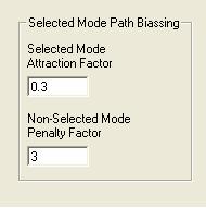
The generalised cost of the selected mode is multiplied by the Selected Mode Attraction Factor and the generalised cost of all the other modes is multiplied by the Non-Selected Mode Penalty Factor.
Back to tutorials On to mode choice models