![]()
![]()
![]()
![]()
![]()
![]()
![]()
![]()
Back to tutorials On to Distribution Models Covered in this section:
What is mode choice?
Mode choice models model the travellers choice of which mode of transport to take, e.g. car, public transport or whatever. They take as input variables about each possible mode of transport that the traveller has available for the trip and gives the proportion of travellers which would use each mode of transport (e.g. 70% by car and 30% by public transport).
Aggregate mode choice
If we have a trip matrix then we can split it into trip matrices for each mode of transport by considering each origin-destination movement (or matrix cell) in turn. The proportion by each mode is calculated and applied to the trip matrix to give the number of trips for each mode. This calculation is then repeated for each origin to destination zone pair in the trip matrix to give the number of trips made by each mode.
Input data
When conducting a Modal Choice exercise there are three key elements. These are discussed below.
Skims
A skim is a matrix containing a variable for each zone to zone movement in the study area. They can either be associated with specific links such as fuel cost or in vehicle time or they can be a cost simply associated with making the journey such as car park costs or waiting time.The intention of the skimming process is to generate O-D pair matrices for each of the skims, i.e. to identify all the variables of travelling from all zones to all zones.
If these variables are attributed to the network, Visual-tm provides the mechanism for generating these matrices. This process is discussed fully in the Assignment Models tutorial.
For a mode choice study you need to generate a set of skims for each mode of transport to be analysed.
Coefficients
In laymans terms, coefficients are weighting factors that tell the mode choice model how much emphasis to place on each associated cost. They can differ greatly from region to region. For example in a very affluent area it is likely that the most important factor when making a mode choice decision is the length of time taken to make the journey whereas in a much poorer area, cost may be the most important factor.The coefficient files themselves are stored in a text format with a file extension of .pdo. They can be viewed and edited using a text-editing package such as Brief, WordPad or Notepad.
In this section of the tutorial we will explain the structure of these files; however, the coefficient values themselves will not be discussed. Coefficient values can be derived with Stated Preference market research. Peter Davidson Consultancy has a wealth of experience in this field and currently holds an extensive library of coefficients that have been obtained through Stated Preference market research.
The coefficients for the CAW market segment are called CoeffMchoiCAW.pdo and are stored in ScenarioCoefficients\Base. Open the file using your text-editing package:
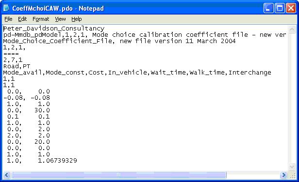
The first four lines are headers and version information that give the purpose of the file and the coefficient file version and the fifth line separates this information from the start of the actual data.
The sixth line gives four numbers 2,7,1,1 (x,y,a,b) where x = No of modes y = No of market segments (attributes) in the skim file. a = No of full sets of coefficients in the file b = No of calibration areas (always set to 1)
The seventh line gives names of the modes in order. This order is important and should be remembered for when attempting the mode choice model run.
The eighth line gives the attribute titles, which should be the same for all modes. Again the order is important and should be the same as the order in the skim files.
The ninth and tenth lines contain information for nested logit models. Currently these values are always set to 1.
The remaining rows have one column of data for each mode.
The eleventh and twelfth rows are scaling factors to scale the relative coefficients to match the observed mode shares. The twelfth row is the scaling factor.
On the thirteenth line the coefficients start. The coefficient of each attribute is given in a column, in the same order as the attributes are listed on line eight. Commas are used to separate the values.
The row following the coefficients should always have as many zeroes on it as there are modes.
The final two rows are Calibration factors. These are output from mode choice calibration and the user should set these to unity to start with.
For use in the multi-mode four stage model, a set of coefficients may appear for each calibration area, where the value on the sixth line described above as a says how many times it is repeated. The section to be repeated is from row 9 onwards. This will be explained in more detail in chapter 22.
When creating your own coefficient file you can either make a copy of an existing one and edit it or start from scratch remembering to keep to the structure described above.
Trip Matrix
The trip matrix holds the number of trips by all modes between each origin and destination. This matrix is to be split by the mode choice model into one matrix for each mode of transport using the logit model. This input trip matrix may be in either CSV or binary ERICA format.Running the matrix model
The first method we will discuss is where the user has a simple trip matrix stored in Comma Separated Variable format and the objective is to split this trip matrix into one matrix for each mode.
The tutorial will now demonstrate how to do this by performing the base year mode split for the test data.
Lets concentrate on the Car Available Work (CAW) market segment. The observed mode split, taken and expanded from market research is:
Mode No. of trips Mode share (%) Car 45499 99.00 PT 459 1.00 Total 45958 100.00 The aim at this stage is to calibrate a model that predicts a mode split very similar to that shown above i.e. it accurately portrays the current situation.
Open the test data if it is not already open. On the main Models menu click Mode Choice and then choose the Matrix option. This opens the Mode Choice form shown below.
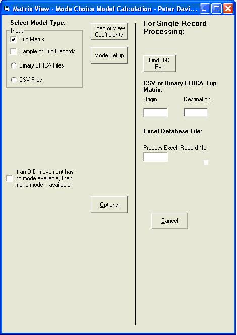
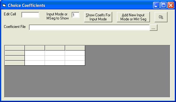
Click the Load or View Coefficients button to open the form below.
Click
for the Coefficient file. The Open File dialogue box appears. Browse to the CoeffMchoiCAW.pdo file stored in ScenarioCoefficients\Base. Select and click Open. This will redisplay the form (click OK to close it):
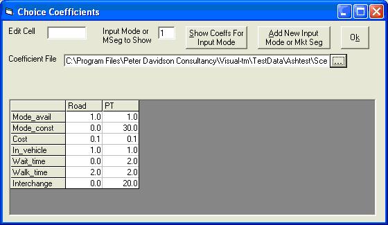
For this type of mode choice run, the model type is a trip matrix in CSV format. Make sure that these box and option buttons (and only these) are selected. There are two modes in the Ashtest project, so enter 2 into the No. of Modes text box. No. of Mkt Segs is always left as 1.
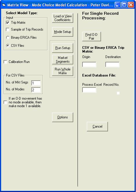
If the Mode Available attribute is set to zero for all the modes for a given O-D pair, the trips will not be allocated to any of the output matrices. This may be prevented, if desired, by clicking the check box labelled If an O-D movement has no mode available, then make mode 1 available. This will assign all the trips for the O-D pair to the first mode. There are no such O-D pairs in this test data set but this can be an issue when for example running a mode choice model on a non car available market segment, depending upon how you have configured your network. Best practice is to code your network so that there is at least one mode available for each o-d movement.
The Mode Setup is not required, as we have already created our coefficient file.
Click Run Setup on the mode choice model calculation form and the form below will open.
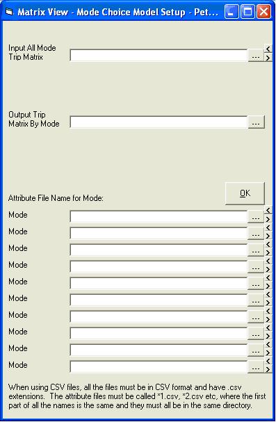
This is the main form where you set the parameters for your model run.
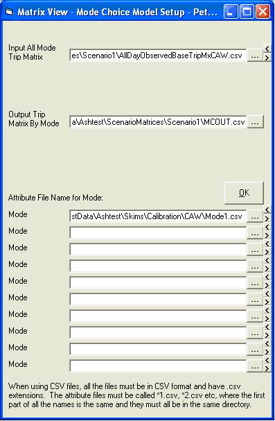
Because we are calculating base mode split we will use the base input trip matrix. This file is called AllDayObserved_AllModeCAW.csv and is stored in ScenarioMatrices\Base. Click
The output trip matrix is specified by the user. Click
We now need to allocate the skim files for each mode we have created. It is essential that the skim files are input in the same order as the modes were set up in the coefficients file i.e. Car; PT.
The skims must all be in the same directory and have names of the form *1.csv, *2.csv etc. These must also be in the correct order and the *1.csv file should be entered in the first skim file text box. The rest do not need to be entered as the program derives their names.
Click the
For a simple trip matrix mode split this form is now completed and should look like this:
Click OK to close the form and save.
Back on the Mode Choice form, click Options to open the Model Options form. On the General tab make sure the number of zones and number of internal zones are set correctly. For the test data these are 66 and 37 respectively. Click OK to close the form.
We are now ready to perform the mode split. To do this click Run Whole Matrix.
Please be aware that running the mode choice model for a very complex network can take 10 or 15 minutes. However in the Ashtest data it should be completed in a matter of seconds.
Once finished, the total numbers of trips allocated to each mode are given on the form.
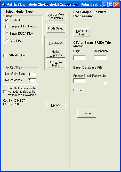
Lets now compare these figures with the observed mode split we mentioned earlier.
Mode Observed Forecast No of trips Mode share No of trips Mode share Car 45499 99.00% 45842.57 99.97% PT 459 1.00% 15.89 0.03% Total 45958 100.00% 45858.46 100.00% As you can see the model predicts a mode split that accurately portrays the observed situation. Therefore our first objective has been met.
Calibration
If the forecast mode share did not match the base then values on the twelfth line of the coefficient file could be changed until the two match.Binary ERICA Inputs
It is possible to run the Mode Choice model with input skim and matrix files that are in Binary ERICA format. In this case all of the skim files need to be entered on the Run Setup form.
Back to tutorials On to Mode Choice Calculators On to Distribution Models